38 Semi-regular PEPS parent Hamiltonians and the four-cut closure
When the virtual group action on the bonds is semi-regular with positive multiplicities, physical bond transformations relate the semi-regular regional ground spaces and parent kernels to those of the regular representation via copy and Fourier coordinates [ 272 , Sections 5 and 7 ] . On regions cut by four boundary seams, intersection and closure identities classify the native parent ground spaces.
38.1 Open contractions on weighted semi-regular graphs
For a region \(R\) in a finite simple graph and an arbitrary alphabet \(X\), regroup the physical incidence labels as one label on each crossing bond, one tail label on each internal bond, and one head label on each internal bond. This is a coordinate bijection using the ordered endpoints and retaining every incidence at the boundary. It is the incidence part of the regional coordinates in [ 272 , Section 6.2 ] and of the bond-endpoint argument in [ 272 , Section 7 ] .
The two internal labels are precisely the physical labels at the ordered tail and head. On a crossing bond, the single retained physical label is the tail label when the tail lies in \(R\), and the head label when the head lies in \(R\).
Each internal edge has exactly two incidences in \(R\), whereas each crossing edge has exactly one. Read these incidences in the coordinate bijection.
Let \(R\) be a region in a finite simple graph. Incident virtual labels split into internal-bond labels and crossing-bond labels. For a finite virtual alphabet \(X\), site coefficients \(A_v\), prescribed crossing labels \(\theta \), and physical configuration \(\sigma \), define the open coefficient by summing the product of the site coefficients over incident assignments whose crossing restriction equals \(\theta \). The physical alphabet may depend on \(v\). These are the finite contraction coordinates used in [ 272 , Sections 6.2–6.3 and 7 ] .
The two factors of the incident-label bijection read exactly the original internal and crossing labels. Prescribing \(\theta \) therefore gives
with each internal assignment counted once. When the physical alphabet is uniformly numbered, enumerating \(X\) into finite indices gives exactly the original numbered open-region coefficient of the same site tensors. No boundary-state equality or Gram identity is a hypothesis.
Partition incident edges into internal and crossing edges and reindex their labels along the resulting bijection. The prescribed crossing condition removes the crossing-label sum. For numbered coefficients, reindex each incident virtual label by the same finite enumeration; the site products and boundary condition are unchanged.
In the regional incidence decomposition underlying [ 272 , Sections 6.2 and 7 ] , for a region \(R\) in a finite simple graph, a product over its incidences equals the product of both endpoint factors on each internal edge, multiplied by the product of the single retained endpoint factor on each crossing edge.
Extending the incidence factors by \(1\) outside \(R\), regrouping the ambient incidence product by edges, and separating internal edges from crossing edges yields the decomposition.
Let \(G\) be finite, \(U:G\to \operatorname {Mat}_X(\mathbb C)\) a representation, \(W\) a virtual weight, and \(R\) a region of a finite simple graph with ordered endpoints. Write \(\kappa =|G|\), and prescribe crossing virtual labels \(\theta _e\). The physical labels are \((\beta _{\partial },\beta _t,\beta _h)\) in crossing, internal-tail, and internal-head coordinates. For \(q:R\to G\), set
Define
These are the regional endpoint factors from the contraction calculation in [ 272 , Sections 6.2 and 7 ] ; the site average is normalized as described in [ 106 ] .
Suppose \(W\) commutes with every \(U(g)\). The open contraction of the averaging sites dressed by \(W\), evaluated at a physical incidence configuration \(\alpha \), equals \(H_R(\theta ,\beta )\), where \(\beta \) is the incidence regrouping of \(\alpha \). Thus regrouping by the coordinate bijection gives exactly the displayed bond formula. The case \(W=I\) gives the ordinary averaging-site coefficients. If the local physical incidence configurations have uniform finite enumerations, the same formula is exactly the numbered open-region coefficient of those enumerated site tensors. The crossing labels are arbitrary throughout. These finite-simple-graph coefficient identities do not assert an equivalence of all open-boundary state spaces.
Fixing the crossing labels and summing only over internal virtual labels, expanding the independent site averages and regrouping their incidence products sums each internal label once, giving \((U(q_h)W)(WU(q_t^{-1}))=W^2U(q_hq_t^{-1})\). Crossing labels are fixed, so their single endpoint factors remain. The incidence bijection reads the physical endpoint labels directly, and finite enumerations reindex the same coefficient sum.
38.1.1 Matching sectors in open weighted regions
For a finite simple graph with edge set \(E\) and ordered endpoints, write \(E_R\) for edges internal to \(R\) and \(\partial E_R\) for edges crossing its boundary. An internal edge \(f=(t,h)\) is indexed in head–tail order. The open contractions below retain arbitrary virtual boundary labels. They give support consequences of the bond transformation in [ 272 , Section 7 ] for the regional parent spaces.
For finite coordinate sets \(X_i\), let \(X=\coprod _iX_i\). The matching-sector coordinate inclusion is \(j:\coprod _i(X_i\times X_i)\hookrightarrow X\times X\), given by \(j(i,a,b)=((i,a),(i,b))\). Its matrix is the matching-sector bond inclusion \(E_X\).
Let \(j:B\hookrightarrow A\) be an injection with \(B\) finite, and let \(E_j(a,b)=\delta _{a,j(b)}\). Then \((E_jx)(j(b))=x(b)\) and \((E_jx)(a)=0\) outside \(j(B)\). Consequently
For any finite set \(E\), the product matrix \(\bigotimes _{f\in E}E_j\) is the coordinate inclusion induced by \(j^E:B^E\hookrightarrow A^E\). In particular, a vector in \(\operatorname {im}\bigotimes _{f\in E}E_X\) vanishes whenever one endpoint pair has different sector labels.
At \(a=j(b)\), the sum \(\sum _c\delta _{a,j(c)}x(c)\) has only the term \(c=b\); outside \(j(B)\) every summand is zero. Conversely, if \(\psi \) vanishes outside \(j(B)\), take \(x(b)=\psi (j(b))\) to prove (6). The product of coordinate indicators is the indicator of equality of the full configurations. For a mismatched bond, each summand in the product inclusion has a zero factor at that bond.
Let \(X\) and \(G\) be finite, \(G\) a group, \(U:G\to \operatorname {Mat}_X(\mathbb C)\) a representation, and \(W\in \operatorname {Mat}_X(\mathbb C)\). Fix virtual labels \(\theta :\partial E_R\to X\) and physical labels \(\sigma :\partial E_R\to X\). For \(q:R\to G\), define
For a regional physical vector \(\psi \), its internal slice \(\mathcal S_{R,\sigma }\psi \) fixes these physical crossing labels and regards the remaining indices as \(\beta :E_R\to X\times X\), with \(\beta _f=(\beta _{h,f},\beta _{t,f})\). If incident endpoint configurations at every vertex are enumerated by bijections \(e_v:X^{\operatorname {Inc}(v)}\cong \{ 0,\ldots ,p-1\} \), the same slice in numbered physical coordinates first uses these bijections to assemble each site index.
Suppose \(W\) commutes with \(U(g)\) for every \(g\in G\). Let \(A\) be the weighted averaging-site family and let \(\mathcal C_R(A)|\theta \rangle \) denote its open contraction with fixed virtual boundary labels \(\theta \). Then
Regrouping the open contraction into crossing endpoints and internal head–tail pairs, the internal virtual sum gives \((U(q_h)W)(WU(q_t^{-1}))=W^2U(q_hq_t^{-1})\). Each crossing edge contributes only its retained endpoint factor from (10). Collecting these factors and the site-average normalization yields (11).
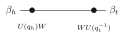 \(=\)

Let \(I\) be finite, \(d_i{\gt}0\), and let \(D_i:G\to \operatorname {Mat}_{d_i}(\mathbb C)\) be representations. Put \(X=\coprod _i\{ 0,\ldots ,d_i-1\} \), \(U(g)=\bigoplus _iD_i(g)\) and \(W=\bigoplus _i d_i^{1/4}I_{d_i}\). Let \(A\) be the weighted averaging-site family, and set \(\psi =\mathcal S_{R,\sigma }\mathcal C_R(A)|\theta \rangle \). For arbitrary \(R,\theta ,\sigma \),
where \(F\) is the full endpoint multiplicity-restoring map with multiplicity \(d_i\) in sector \(i\), and \(U'(g)=\bigoplus _i(D_i(g)\otimes I_{d_i})\). The coefficients \(c_R\) still use the original \(U,W,\theta ,\sigma \).
The block-scalar matrix \(W\) commutes with \(U(g)\), and \(W^2U(g)=\bigoplus _i\sqrt{d_i}\, D_i(g)\). Applying coherent multiplicity restoration to (11), with coherent coefficients \(c_R(\theta ,\sigma ;q)\) and bond labels \(q_hq_t^{-1}\), gives both product support and (13). Only internal bonds are acted on, so the crossing factors remain those in (10).
Use the representations and positive dimensions of Theorem 38.1.1.5, and suppose each site’s incident endpoint configurations have a bijection \(e_v:X^{\operatorname {Inc}(v)}\cong \{ 0,\ldots ,p-1\} \). Let \(A\) be the resulting weighted averaging tensor in these numbered physical coordinates. For any region \(R\), any crossing physical labels \(\sigma \), and every \(\psi \in \mathcal G_R(A)\),
Thus \(\psi \) vanishes at every physical configuration whose two endpoint labels on some internal edge belong to different sectors.
The open contractions \(\mathcal C_R(A)|\theta \rangle \) span \(\mathcal G_R(A)\). Reindexing their virtual and physical labels identifies their slices with those of Theorem 38.1.1.5. The slice is linear and the product inclusion range is a subspace, so support extends to every vector in \(\mathcal G_R(A)\). At a given physical configuration, choosing its own crossing labels for \(\sigma \) and regrouping the remaining endpoints shows that a mismatched internal sector forces a zero coefficient by Theorem 38.1.1.2.
Let \(A\) and the endpoint enumerations be as in Theorem 38.1.1.6. Suppose that for every edge \(f=(t,h)\) there is a parent region \(R_i\) containing both \(t\) and \(h\). If \(\psi \in \mathcal P_{\mathcal R}(A)\), then \(\psi \) vanishes whenever one physical bond has different endpoint sector labels. Equivalently, regrouping the physical endpoint coordinates by bonds gives a vector \(\widetilde\psi \) satisfying
Neither irreducibility nor completeness of the block representations is required.
Choosing a region containing both endpoints of a mismatched bond and fixing the exterior physical configuration places the resulting regional slice in \(\mathcal G_{R_i}(A)\) by the parent condition, so Theorem 38.1.1.6 makes its coefficient zero. Reassembling the regional and exterior indices gives the original coefficient of \(\psi \). The image of the coordinate inclusion \(j^E\) consists exactly of configurations with matching sectors on every bond, since each matched pair is determined by its shared sector and its two internal labels. Equation (6) therefore turns the vanishing condition into (15).
38.2 Regional support of physical bond transformations
The bond transformation of [ 272 , Section 7 ] acts on head–tail endpoint pairs; its regional blocks, including the one-ended factors on crossing edges, determine the product support of regional parent spaces. Throughout the graph statements, \(\Gamma \) is a finite simple graph with ordered vertices. For a region \(R\), write \(E_R\) for its internal edges, \(\partial E_R\) for its crossing edges, and \(E_{R^c}\) for its exterior edges. An edge \(f=(t,h)\) has \(t{\lt}h\).
38.2.1 Products, coordinate slices, and multiplicity maps
Let \(B,E\) be finite sets, with matrices \(F_b:\mathbb {C}^X\to \mathbb {C}^Y\) and \(K_f:\mathbb {C}^P\to \mathbb {C}^Q\). Their mixed product has coefficients
When \(X,P\) are finite, its action is \((\mathcal M(F,K)\psi )(\tau ,\beta ) =\sum _{\sigma ,\alpha }\mathcal M(F,K)_{(\tau ,\beta ),(\sigma ,\alpha )} \psi (\sigma ,\alpha )\).
The adjoint satisfies \(\mathcal M(F,K)^\dagger =\mathcal M(F^\dagger ,K^\dagger )\). Assume \(X,P\) are finite. For a finite index set \(A\), weights \(w_a\), and factor vectors \(x_{b,a}\in \mathbb {C}^X\), \(y_{f,a}\in \mathbb {C}^P\), one has
Let \(S,X,Y\) be finite and \(F:\mathbb {C}^X\to \mathbb {C}^Y\) a matrix. For \(\psi \in \mathbb {C}^{Y^S}\), define \(\psi _{v,\tau }(s)=\psi (\tau [v\mapsto s])\). Then
In the forward implication \(Y\) need not be finite. For any matrix \(P:\mathbb {C}^Y\to \mathbb {C}^Y\) with \(Y\) finite, if \(P\psi _{v,\tau }=\psi _{v,\tau }\) for every \(v,\tau \), then \(P^{\otimes S}\psi =\psi \); idempotence of \(P\) is unnecessary. The assertions allow empty sets and impose no rank condition on \(F\).
A slice of \(F^{\otimes S}\chi \) is a linear combination of columns of \(F\), with coefficients obtained by contracting all other factors. For the converse choose a linear right inverse of \(F\) on its image and extend it to \(L:\mathbb {C}^Y\to \mathbb {C}^X\). Thus \(FL\) fixes every slice. Applying \(FL\) at one coordinate fixes \(\psi \). Induction over finite subsets of \(S\) shows that applying it at all coordinates also fixes \(\psi \). Consequently \(F^{\otimes S}(L^{\otimes S}\psi )=(FL)^{\otimes S}\psi =\psi \). The same induction proves the assertion about an arbitrary \(P\).
Let \(I\), the sets \(X_i\), and the multiplicity sets \(M_i\) be finite. Put \(X=\coprod _iX_i\), \(Y=\coprod _i(X_i\times M_i)\), and \(m_i=|M_i|\). For \(y=(i,a,u)\in Y\), define \(b(y)=(i,a)\) and \(c(y)=(i,u)\). Set
Whenever the first case occurs, \(M_i\) contains \(u\), so \(m_i{\gt}0\).
Let \(F=E_YJE_X^\dagger :\mathbb {C}^{X\times X}\to \mathbb {C}^{Y\times Y}\) be the full endpoint multiplicity map, where \(J|i,a,b\rangle =m_i^{-1/2}\sum _{u\in M_i}|i,(a,u),(b,u)\rangle \) and an empty sum is zero. Its coefficient and action formulas are
Also \(a(y,z)=a(z,y)\). These formulas require neither nonempty multiplicity sets nor support conditions on the input vectors. More generally, for a coordinate inclusion \(j:B\hookrightarrow A\) with \(A\) finite, its inclusion matrix satisfies \((E_j^\dagger \phi )(i)=\phi (j(i))\).
The adjoint of a coordinate inclusion selects its included coordinates. For equal sectors, the multiplicity map retains equal copy labels and multiplies by \(m_i^{-1/2}\); for unequal sectors its coefficient is zero. This proves the formula for \(F\phi \). Evaluating it on coordinate vectors gives (22); the product of its coordinate indicators selects the single input configuration in (24). Equal copy labels have equal sectors and hence equal normalizations, proving symmetry.
Assume every \(M_i\) is nonempty. Let \(E_X\) be the matching-sector inclusion and let \(\mathcal F=F^{\otimes E}\) for a finite set \(E\). Then \(FF^\dagger F=F\). For \(\psi \in \operatorname {im}E_X^{\otimes E}\) and \(\phi \in \operatorname {im}\mathcal F\),
Since \(F^\dagger F=E_XE_X^\dagger \) and \(E_X^\dagger E_X=I\), the factorization \(F=E_YJE_X^\dagger \) gives \(FF^\dagger F=F\). Products respect multiplication. Write \(\psi =E_X^{\otimes E}\chi \) and \(\phi =\mathcal F\eta \), respectively, and cancel the corresponding local factors.
38.2.2 One-ended boundary transformations
For weights \(\lambda _i\in \mathbb {C}\) and a fixed exterior endpoint \(z\in Y\), define \(B_z^\lambda :\mathbb {C}^X\to \mathbb {C}^Y\). For \(y=(i,a,u)\), put
Write \(B_z=B_z^1\) for unit weights.
For arbitrary matrices \(T_i\) on \(X_i\), write \(M=\bigoplus _iT_i\), \(M^{[m]}=\bigoplus _i(T_i\otimes I_{M_i})\), and \(M_\lambda =\bigoplus _i\lambda _iT_i\). For \(x\in X\) and \(y,z\in Y\),
The entries of \(B_z\) are real, hence \(B_z^\dagger =B_z^{\mathsf T}\). A block scalar may be read from either index: \((M_\lambda )_{x,r}=\lambda _{i(x)}M_{x,r} =\lambda _{i(r)}M_{x,r}\).
The block-diagonal and identity factors force the sector and copy coordinates in the sum. The remaining matrix entry is that of \(T_i\), multiplied by \(\lambda _i m_i^{-1/2}\). Transposing the block matrices exchanges the two contraction formulas. The action formula follows by summing the single surviving input coordinate in (27). Its unit-weight coefficient is real. Off-block entries vanish; on a block, the row and column sector labels agree.
Suppose \(\lambda _i\ne 0\) for every \(i\). With the preceding notation,
Independently of these weights, if every \(M_i\) is nonempty then
for arbitrary matrices \(T_i\) on \(X_i\), where \(\operatorname {vec}(T)(x,r)=T_{x,r}\). In particular, for representations \(D_i\) of dimensions \(d_i\), \(D=\bigoplus _iD_i\) and \(W=\bigoplus _i d_i^{1/4}I_{d_i}\) satisfy \(WD(g)=D(g)W=\bigoplus _i d_i^{1/4}D_i(g)\).
Applying (29) with unit weights and using \(B_z^\dagger =B_z^{\mathsf T}\) gives the adjoint boundary formulas, since reading the block weight from the fixed \(y\) index permits cancellation of \(\lambda _{i(y)}\). Because the repeated matrix-entry vector in (33) is \(F\) applied to the square-root-weighted block vector and the block-diagonal input lies in the matching-sector range, \(F^\dagger F=E_XE_X^\dagger \) yields the internal adjoint identity. The fourth-root identities follow by multiplying block-scalar matrices on the left and on the right.
38.2.3 Physical coordinates and regional operator blocks
Choose bijections \(e_v:X^{\operatorname {Inc}(v)}\to \{ 0,\ldots ,p-1\} \). Decoding a numbered configuration and grouping its endpoint labels gives a bijection \(j_e:\{ 0,\ldots ,p-1\} ^V\to (X\times X)^E\). The pair on \(f=(t,h)\) is \((x_{h,f},x_{t,f})\). Its coefficient-space isomorphism is \(J_e\psi (\beta )=\psi (j_e^{-1}\beta )\). Regionally the same regrouping gives
The inverse assigns each crossing label to its inside incidence, and each internal pair to its head and tail incidences, before applying the corresponding \(e_v\). If \(\sigma \) is a numbered exterior configuration, let \(\gamma ^e_R(\sigma )_f\) be its endpoint label outside \(R\): the head label when \(t\in R\), and the tail label when \(h\in R\).
Let \(e^X,e^Y\) enumerate incident configurations of \(X,Y\), respectively, and let \(F:\mathbb {C}^{X\times X}\to \mathbb {C}^{Y\times Y}\). Define the matrix \(N_F\) between the numbered physical spaces by
The matrix \(N_F\) is the matrix of \(F^{\otimes E}\) with rows relabelled by \(j_{e^Y}\) and columns by \(j_{e^X}\). Thus \(J_{e^Y}N_F=F^{\otimes E}J_{e^X}\) and \(N_F^\dagger =N_{F^\dagger }\), where the latter operator exchanges the two enumerations.
The product coefficients agree by definition, and reindexing the matrix-vector sum by the bijection \(j_{e^X}\) gives the intertwining identity. Conjugating each factor in (35) proves the adjoint identity.
For a matrix \(M\) between global numbered physical spaces, define its regional block by \(M_R[\tau ,\sigma ]_{y,x}=M_{y\cup \tau ,x\cup \sigma }\), where \(x,y\) are configurations on \(R\), and \(\sigma ,\tau \) are configurations on \(R^c\). Write \(S_{R,\sigma }\psi (x)=\psi (x\cup \sigma )\) for an exterior slice.
For every exterior output configuration \(\tau \),
Let \(A,B\) be tensors on the same graph, possibly with different physical dimensions, and let \(\mathcal R=(R_i)_{i\in \iota }\) be any region family. If \(M_{R_i}[\tau ,\sigma ]\mathcal G_{R_i}(A) \subseteq \mathcal G_{R_i}(B)\) for every \(i,\tau ,\sigma \), then \(M\mathcal P_{\mathcal R}(A)\subseteq \mathcal P_{\mathcal R}(B)\). Here \(\mathcal P_{\mathcal R}(A)\) consists of vectors whose every exterior slice on \(R_i\) belongs to \(\mathcal G_{R_i}(A)\).
Splitting the global input-coordinate sum into its regional and exterior coordinates gives (36). Taking the adjoint exchanges input and output configurations. If \(\psi \in \mathcal P_{\mathcal R}(A)\), every summand in (36) lies in \(\mathcal G_{R_i}(B)\) by the assumed block inclusion. This space is closed under sums, proving all target parent constraints.
Fix exterior configurations \(\tau ,\sigma \), and put \(\gamma _Y=\gamma _R^{e^Y}(\tau )\), \(\gamma _X=\gamma _R^{e^X}(\sigma )\). The matrix on the inside endpoint of a crossing edge is
Decode the exterior endpoint labels as \(\tau _{h,f},\tau _{t,f}\) and \(\sigma _{h,f},\sigma _{t,f}\). Define the exterior scalar and, for the multiplicity map, its crossing-indicator factor by
For any weights \(w_f\), the edge partition gives \(\prod _{f\in E}w_f=(\prod _{f\in E_{R^c}}w_f) (\prod _{f\in \partial E_R}w_f)(\prod _{f\in E_R}w_f)\). Accordingly, the blocks of the global bond operator satisfy
Since every edge has zero, one, or two endpoints in \(R\), the product in (35) separates into these three cases. The first contributes \(c_{R,F}\), the second gives (40), and the third retains \(F\) on its head–tail pair. Regional regrouping places these factors in the two coordinate families of \(\mathcal M\).
For the multiplicity map \(F\) and any \(z,y\in Y\), \(r,x\in X\),
Thus \(C_f=\delta _{b(\gamma _Y(f)),\gamma _X(f)}B_{\gamma _Y(f)}\) in either orientation, and
38.2.4 Open contractions and their product support
Let \(G\) and \(X\) be finite, \(U:G\to \operatorname {Mat}_X(\mathbb {C})\) a representation, and \(W\) a matrix on \(X\). For \(q:R\to G\), define
With virtual boundary labels \(\theta \in X^{\partial E_R}\), put
This is the coherent open bond vector in crossing and internal head–tail coordinates.
Let \(a_v^{U,W}(\eta ,\xi )\) be the dressed averaging site. In a chosen incident enumeration \(e\), the numbered tensor is \(A(U,W,e)_v(\eta ,s)=a_v^{U,W}(\eta ,e_v^{-1}(s))\), with virtual labels numbered by a bijection \(X\cong \{ 0,\ldots ,|X|-1\} \). Dressing by \(W=I\) gives the unweighted averaging site. Define the open bond space by \(\mathcal H_R(U,W)=\operatorname {span}_{\mathbb {C}} \{ H_R^{U,W}(\theta ):\theta \in X^{\partial E_R}\} \).
Suppose \(WU(g)=U(g)W\) for every \(g\). Then
In particular, \(J_{e,R}\phi \in \mathcal H_R(U,W)\) if and only if \(\phi \in \mathcal G_R(A(U,W,e))\). More generally, for any site family \(a_v(\eta ,\xi )\), numbering its virtual and physical labels leaves every internal slice of each open column unchanged: with the same \(\theta \) and fixed crossing physical labels \(\sigma \), the numbered and incidence contractions give the same function of internal head–tail pairs.
Decoding the numbered labels and applying the open contraction formula shows that the inverse regional coordinate map puts each crossing, head, and tail label back at its original incidence, proving the column equality in (53). Open columns span \(\mathcal G_R\), and their boundary numberings are bijective, so their images span \(\mathcal H_R\). Injectivity of \(J_{e,R}\) gives the membership equivalence. The final assertion follows directly by decoding the virtual boundary labels in the finite contraction sum and then fixing the crossing physical coordinates; it needs no representation or commutation hypothesis.
Let \(A\) be any tensor with incident enumeration \(e\) by a finite endpoint set \(X\), and let \(F:\mathbb {C}^Z\to \mathbb {C}^{X\times X}\) with \(Z\) finite. Suppose every edge is internal to some region \(R_i\). Assume that, for every \(i\), every crossing physical configuration \(\sigma \), and every \(\phi \in \mathcal G_{R_i}(A)\),
Then \(J_e\psi \in \operatorname {im}F^{\otimes E}\) for every \(\psi \in \mathcal P_{\mathcal R}(A)\). The coordinate identity used here is the following. Fix global bond labels \(\beta \) and an internal edge \(f\in E_R\). Let \(\sigma \) be their crossing labels inside \(R\), and let \(\tau \) be their numbered exterior configuration. For every endpoint pair \(s\),
Updating an internal edge changes only its two inside incidences; it leaves all crossing and exterior incidences fixed. This proves (55). For each edge \(f\), choose a covering region \(R_i\). The parent condition places \(S_{R_i,\tau }\psi \) in \(\mathcal G_{R_i}(A)\), so (54) and the forward implication of (18) put its \(f\)-slice in \(\operatorname {im}F\). By (55) this is the global \(f\)-slice, so the reverse implication of (18) across all edges places \(J_e\psi \) in \(\operatorname {im}F^{\otimes E}\).
Let \(U:G\to \operatorname {Mat}_X(\mathbb {C})\) be a representation of a finite group, let \(W\) commute with every \(U(g)\), and let \(F:\mathbb {C}^Z\to \mathbb {C}^{X\times X}\), with \(X,Z\) finite. Suppose \(\operatorname {vec}(W^2U(g))\in \operatorname {im}F\) for every \(g\). Every internal slice of every open column, with arbitrary virtual boundary labels, belongs to \(\operatorname {im}F^{\otimes E_R}\). The same holds for every \(\phi \in \mathcal G_R(A(U,W,e))\). If every edge is internal to a member of \(\mathcal R\), then
Choose \(x_g\) with \(Fx_g=\operatorname {vec}(W^2U(g))\). For each internal slice use the preimage
where \(c_R\) retains all boundary factors and the averaging normalization. Applying \(F^{\otimes E_R}\) term by term gives the weighted slice formula. Numbered and incidence slices agree, and the regional range is spanned by open columns, so the inclusion extends by linearity. Theorem 38.2.4.4 then proves (56).
Let \(d_i{\gt}0\) and let \(D_i:G\to \operatorname {Mat}_{d_i}(\mathbb {C})\) be representations of a finite group. Put \(U'(g)=\bigoplus _i(D_i(g)\otimes I_{d_i})\), and let \(F\) restore multiplicity \(d_i\) on the full endpoint pairs. Every internal slice of each open column for the unweighted averaging tensor of \(U'\) lies in \(\operatorname {im}F^{\otimes E_R}\). This also holds for each vector in the numbered regional range \(\mathcal G_R(A(U',I,e))\). For any edge-covering family \(\mathcal R\),
Neither irreducibility nor unitarity of the \(D_i\) is assumed.
When each target slice is expanded with its own boundary coefficients \(c_R^{U',I}(\theta ,\sigma ;q)\), coherent multiplicity restoration sends the internal factors \(\operatorname {vec}(\bigoplus _i\sqrt{d_i}\, D_i(q_hq_t^{-1}))\) to \(\operatorname {vec}(U'(q_hq_t^{-1}))\), while retaining these same coefficients. This provides a preimage for each target open slice. Linear combinations give all regional vectors; edge coverage and Theorem 38.2.4.4 give (58).
38.3 Open contractions with native edge orientations
Let \(\Gamma =(V,E)\) be a finite simple graph with ordered vertices. Write an ordered edge as \(e=(t,h)\), with \(t{\lt}h\), and let \(o:E\to \{ 0,1\} \) specify its orientation: \(o_e=0\) means \(t\to h\) and \(o_e=1\) means \(h\to t\). The ordering of vertices is used only for coordinates. The physical pair on an edge is always ordered as \((x_h,x_t)\), even when the native arrow is reversed. For \(R\subseteq V\), denote its internal, crossing, and exterior edges by \(E_R\), \(\partial E_R\), and \(E_{R^c}\). For a region family \(\mathcal R\), write \(\mathcal P_{\mathcal R}(A)\) for the physical vectors whose every slice on each \(R\in \mathcal R\) belongs to the regional contraction range of \(A\). These conventions extend the bond transformations of [ 272 , Section 7 ] to the rightward and downward arrows of a torus.
38.3.1 Averaging tensors and unrestricted regional boundaries
An incidence \((v,e)\) is a native tail when \(v=t\) and \(o_e=0\), or when \(v=h\) and \(o_e=1\). Thus the ordered first incidence is a native tail exactly when \(o_e=0\), and the ordered second incidence exactly when \(o_e=1\).
Let \(G\) be finite, \(U:G\to \mathrm{GL}(\mathbb {C}^X)\) a representation, and \(W\) a matrix on \(\mathbb {C}^X\). For virtual and physical incidence labels \(\eta ,\sigma :\operatorname {Inc}(v)\to X\), set
A bijection \(e_v:X^{\operatorname {Inc}(v)}\to \{ 0,\ldots ,p-1\} \) numbers the physical indices. Its coefficient at \(s\) is \(A^{U,W,o}_v(\eta ,e_v^{-1}(s))\). Fix any numbering of \(X\) on the virtual bonds. If every \(o_e=0\), this is the ordered dressed averaging tensor. No symmetry of \(W\) is required. The normalization is the group-average normalization of [ 106 ] .
Fix \(q:R\to G\). On an internal edge \(e=(t,h)\) define
For a crossing edge, let \(v\) be its retained vertex, \(\theta \) its virtual boundary label, and \(x\) its retained physical label. Put \(B_e(q;\theta ,x)=(WU_{q_v^{-1}})_{\theta ,x}\) when \(v\) is the native tail, and \(B_e(q;\theta ,x)=(U_{q_v}W)_{x,\theta }\) otherwise. For arbitrary \(\theta \in X^{\partial E_R}\), define
Here \(z_e=(x_h,x_t)\) and \(x\) lists the retained crossing endpoints. Setting \(o=0\) recovers each ordered boundary factor, internal factor, open vector, and open span.
Assume \(WU_g=U_gW\) for every \(g\). Let \(\mathcal C_R\) be the open contraction of the tensors (61), and let \(J_R\) regroup its physical incidences into crossing labels and ordered internal pairs. Then
These identities hold before or after numbering physical and virtual labels. In particular, \(\psi \in \operatorname {im}\mathcal C_R\) exactly when \(J_R\psi \in \mathcal S_R(U,W,o)\). The boundary coefficients may be arbitrary linear combinations of all \(\theta \), including entangled boundary vectors.
Expanding the normalized group average separately at every vertex yields the factor \(|G|^{-|R|}\) and the sum over \(q:R\to G\), after which we regroup the incidence product by internal and crossing edges. Summation over one internal virtual index gives either \((U_{q_h}W)(WU_{q_t^{-1}})\) or \((U_{q_t}W)(WU_{q_h^{-1}})\) with the physical indices interchanged. Commutation with \(W\) gives (64). Each crossing edge retains its original \(\theta _e\), giving (65); commuting the scalar products also gives the internal-first form of the same sum. The bijections of incidence and numbered labels preserve every finite sum. Finally, the regional range is the span of all its boundary columns, proving (68).
On \(\mathbb {C}^{X^{\operatorname {Inc}(v)}}\), define
Matrix multiplication gives \(\rho _v^o(1)=1\) and \(\rho _v^o(gh)=\rho _v^o(g)\rho _v^o(h)\). At a tail this follows from \((U_{(gh)^{-1}})^T=(U_{g^{-1}})^T(U_{h^{-1}})^T\). Thus these matrices act as a representation by multiplication on coefficient vectors. If \(E_v\) changes numbered virtual coefficients to incidence coefficients, the numbered representation is \(E_v^{-1}\rho _v^o(g)E_v\).
The local coefficient map of \(A^{U,1,o}_v\) is \(\Pi _v=|G|^{-1}\sum _g\rho _v^o(g)\), and is \(G\)-injective. With physical numbering \(P_v\) and virtual numbering \(E_v\), its local map is \(P_v\Pi _v E_v\) and is \(G\)-injective for \(E_v^{-1}\rho _v^o E_v\). This assertion needs neither unitarity nor semi-regularity of \(U\).
Comparing (61) at \(W=1\) with (71) coefficient by coefficient identifies the local map with \(\Pi _v\). The group average satisfies \(\Pi _v\rho _v^o(g)=\Pi _v\) and fixes every invariant vector. Hence its restriction to the invariant subspace is injective. The invertible coordinate changes \(P_v,E_v\) preserve both assertions.
38.3.2 Internal support and regional blocks
Let \(F:\mathbb {C}^Z\to \mathbb {C}^{X\times X}\). Assume both coefficient vectors of \(W^2U_g\) and \((W^2U_g)^T\) belong to \(\operatorname {im}F\) for every \(g\). Then each \(I_e(q)\) belongs to \(\operatorname {im}F\). Assume also \(WU_g=U_gW\). Fixing the physical crossing labels \(x\) in an open vector leaves
This holds for every vector in the regional range after taking its internal physical slice. If a region family \(\mathcal R\) contains both endpoints of every edge in some member, every vector in its parent space \(\mathcal P_{\mathcal R}(A^{U,W,o})\) lies, after regrouping, in \(\operatorname {im}F^{\otimes E}\).
Each orientation selects one of the two assumed matrix orders. Choosing a preimage under \(F\) for every \(I_e(q)\) and taking their product with the scalar coefficient in (72) produces a vector whose image under \(F^{\otimes E_R}\) is the displayed sum. Span closure proves the assertion for every regional vector. For a global parent vector, choose a region containing the endpoints of a prescribed edge. Every one-edge slice then belongs to \(\operatorname {im}F\). The product-range criterion gives the full \(E\)-fold range.
For \(F_e:\mathbb {C}^{X\times X}\to \mathbb {C}^{Y\times Y}\), define \(M(F)=\bigotimes _{e\in E}F_e\), expressed in the numbered site coordinates through the incidence-to-bond bijections. Thus \(M(F)_{\tau ,\sigma }=\prod _eF_e((\tau _h,\tau _t),(\sigma _h,\sigma _t))\) in bond coordinates. Fix exterior endpoint labels \(\gamma _Y,\gamma _X\). On a crossing edge put
For fixed exterior physical configurations \(\tau ,\sigma \), let \(c_R(F;\tau ,\sigma )\) be the product of their matrix coefficients on all \(e\in E_{R^c}\).
The block obtained by fixing exterior output \(\tau \) and input \(\sigma \) satisfies
where \(\gamma _Y,\gamma _X\) are the crossing endpoint labels determined by \(\tau ,\sigma \), and \(J_{X,R},J_{Y,R}\) regroup regional coordinates.
With compatible finite endpoint alphabets, \(M(F)^\dagger =M(F^\dagger )\), \(M(F)M(L)=M((F_eL_e)_e)\), and \(M((1)_e)=1\). In particular, \(F_eL_e=1\) on every edge implies \(M(F)M(L)=1\).
Conjugation distributes over each coefficient product. For composition, the sum over the intermediate site configuration is, under the bond-coordinate bijection, a sum over independent intermediate edge labels. It factors into the products \(F_eL_e\). The product of edgewise Kronecker deltas is the delta of the complete configuration, proving the identity assertion.
38.4 Coordinate changes with native edge orientations
Continue with the incidence and bond coordinates of Section 38.3. The matrix on a reversed edge is the entrywise conjugate of the matrix on an unreversed edge. This conjugation follows from exchanging the two physical endpoints; it does not require real representation matrices.
For a matrix \(Q:\mathbb {C}^X\to \mathbb {C}^Y\), put \(T(Q)=Q\otimes \overline Q\) on ordered head–tail pairs, and let \(S_X,S_Y\) exchange their two coordinates. Then \(T(\overline Q)=S_YT(Q)S_X\) and, for every matrix \(M\) on \(\mathbb {C}^X\),
Here \(\operatorname {vec}(M)(a,b)=M_{a,b}\).
The coefficient of \(T(Q)\) is \(Q_{a,c}\overline{Q_{b,d}}\). Exchanging both endpoint pairs gives \(\overline{Q_{a,c}}Q_{b,d}\), which is \(T(\overline Q)_{(a,b),(c,d)}\). Summing this coefficient against \(M_{d,c}\) gives \((QMQ^\dagger )_{b,a}\).
Set \(Q_e=Q\) if \(o_e=0\) and \(Q_e=\overline Q\) if \(o_e=1\). The internal bond matrix is \(T_e(Q)=Q_e\otimes \overline{Q_e}\). On a crossing edge \(e=(t,h)\), set \(B_{e,R}(Q)=\overline{Q_e}\) when \(t\in R\), and \(B_{e,R}(Q)=Q_e\) when \(h\in R\). Define
The corresponding global matrix in numbered site coordinates is \(M_o(Q)=M((T_e(Q))_e)\).
If \(AB=1\), then \(\overline A\, \overline B=1\). Consequently \(QQ^\dagger =1\) implies \(T_R^o(Q)T_R^o(Q^\dagger )=1\) for every region and orientation.
Taking entrywise conjugates of the finite sums defining \(AB\) gives \(\overline A\, \overline B=1\). Applying this identity to each \(Q_e\), its conjugate on a retained tail, and the two factors of every internal pair, and multiplying the independent boundary and internal tensor factors proves the regional assertion.
Suppose \(Q^\dagger Q=1\) and \(U,L\) are representations satisfying \(L_g=QU_gQ^\dagger \). For \(W=1\), internal factors obey \(T_e(Q)I_e^U(q)=I_e^L(q)\), while crossing factors obey
The internal identity only uses \(L_g=QU_gQ^\dagger \). Put \(K_R(Q)_{a,\theta } =\prod _{e\in \partial E_R}B_{e,R}(Q)_{a_e,\theta _e}\). Then
At a native head, \(L_gQ=QU_g\), and at a native tail, \(Q^\dagger L_g=U_gQ^\dagger \), with conjugates as specified by \(B_{e,R}(Q)\), which gives (79). Internal factors follow by conjugating the relative representation matrix, using (77) on reversed edges. Applying these identities inside (65) and factoring the independent boundary sums yields (80). Linearity gives (81) and the forward range inclusion. At \(g=1\), the representation identity gives \(1=L_1=QQ^\dagger \). The reverse coordinate change \(Q^\dagger \) therefore satisfies the same hypotheses, and cancellation proves (82).
For fixed crossing exterior labels \(\gamma _Y,\gamma _X\), put
The mixed product of crossing blocks and internal coordinate matrices is \(b_R(Q;\gamma _Y,\gamma _X)T_R^o(Q)\). Under the hypotheses of Theorem 38.4.4, every exterior block of \(M_o(Q)\) sends the regional range for \(A^{U,1,o}\) into that for \(A^{L,1,o}\). Thus, for every region family \(\mathcal R\),
No coverage condition is needed for this inclusion.
A crossing coefficient of \(Q_e\otimes \overline{Q_e}\) factors into its fixed exterior entry and its retained endpoint entry, and taking their product gives (85). By (76), each global block is \(c_Rb_RJ_{Y,R}^{-1}T_R^o(Q)J_{X,R}\). Equations (68) and (82) show that this block preserves the required regional range. Each output slice of a global vector is a sum of such blocks applied to its input slices, proving (86).
If \(QQ^\dagger =1\), then \(M_o(Q)M_o(Q^\dagger )=1\) on the full target physical space. If \(Q^\dagger Q=1\), then \(M_o(Q)\) is injective on the full source physical space.
Each edge factor and its inverse cancel, as do the conjugated factors on reversed edges, so their global product cancels by Theorem 38.3.2.4. Applying the same identity to \(Q^\dagger \) yields a left inverse under \(Q^\dagger Q=1\) and hence injectivity.
If \(Q^\dagger Q=1\) and \(L_g=QU_gQ^\dagger \) for representations \(U,L\), then for every \(\mathcal R\),
These parent spaces have equal dimension. For a finite region family, let \(H_U,H_L\) be sums of positive regional interactions whose kernels are exactly the respective regional contraction ranges. Then \(M_o(Q)\ker H_U=\ker H_L\).
Evaluating the intertwining identity at \(1\) gives \(QQ^\dagger =1\). Applying the block inclusion in both directions and cancelling the global coordinate matrices shows that the restriction of \(M_o(Q)\) is bijective, which gives equal dimension. Positivity identifies each Hamiltonian kernel with the intersection of its regional parent conditions, giving the kernel assertion.
Under the hypotheses of Theorem 38.4.8, define \(E_Q^o:\mathcal P_{\mathcal R}(A^{U,1,o}) \simeq \mathcal P_{\mathcal R}(A^{L,1,o})\) to be the restriction of \(M_o(Q)\). Its inverse is the restriction of \(M_o(Q^\dagger )\).
38.5 Positive multiplicities and complete canonical parent spaces
Fix a finite group \(G\), a finite ordered simple graph, and a finite family of matrix representations \(D_i:G\to \operatorname {Mat}_{d_i}(\mathbb {C})\). Write \(X=\coprod _i\{ 0,\ldots ,d_i-1\} \) and \(X_m=\coprod _i(\{ 0,\ldots ,d_i-1\} \times \{ 0,\ldots ,m_i-1\} )\). An edge is written \(f=(t,h)\); physical bond coordinates are ordered head–tail. The construction extends the dimension multiplicities in [ 272 , Section 7 ] to arbitrary positive integers \(m_i\). Irreducibility of \(D_i\) is not required.
38.5.1 Copy weights and arbitrary open boundaries
Define \(D(g)=\bigoplus _iD_i(g)\), \(D^{[m]}(g)=\bigoplus _iD_i(g)\otimes I_{m_i}\), and \(W_m=\bigoplus _i m_i^{1/4}I_{d_i}\). Taking \(m_i=d_i\) gives dimension multiplicity restoration and the fourth-root dimension weight. Let \(A_m\) be the averaging tensor for \(D\) with virtual weight \(W_m\), and let \(B_m\) be the unweighted averaging tensor for \(D^{[m]}\). Their site averages use the same factor \(|G|^{-1}\).
For every \(g\in G\),
Within each diagonal block, the scalar weight \(m_i^{1/4}\) commutes with \(D_i(g)\) and satisfies \((m_i^{1/4})^2=\sqrt{m_i}\).
Let \(F_m:\mathbb {C}^{X\times X}\to \mathbb {C}^{X_m\times X_m}\) be the supported normalized copy map. For \(y=(i,a,c)\), write \(\pi y=(i,a)\), and set \(\alpha _m(y,z)=m_i^{-1/2}\) when \(y,z\) have sector \(i\) and the same copy label, and zero otherwise. Its one-ended map with fixed exterior output \(z\) is \(B_z(y,x)=\alpha _m(y,z)\delta _{\pi y,x}\). For a region \(R\), let \(E_R\) be its internal edges and \(\partial E_R\) its crossing edges. Given \(\gamma :\partial E_R\to X_m\), define
The numbered regional matrix is obtained by regrouping the site labels into these crossing endpoints and internal head–tail pairs. The dimension-multiplicity versions are obtained by setting \(m=d\).
Assume \(m_i{\gt}0\). Fix \(q:R\to G\). Denote the internal bond factors of \(A_m,B_m\) by \(a_f(q),b_f(q)\), and the crossing factors with virtual label \(\theta \) by \(a_f(q;\theta ),b_f(q;\theta )\). For an internal edge, \(F_ma_f(q)=b_f(q)\) and \(F_m^\dagger b_f(q)=a_f(q)\). For a crossing edge and exterior output \(z\in X_m\),
where \(w_y=m_i^{1/4}\) for \(y\) in sector \(i\). These formulas hold for both crossing orientations; each crossing retains exactly one fourth-root weight.
The internal factor is \(W_m^2D(q_hq_t^{-1})\). Equation (89) gives \(\sqrt{m_i}\) in each block, canceled by the normalized copy map. Its adjoint sums \(m_i\) equal-copy terms with coefficient \(m_i^{-1/2}\), recovering the same factor. At a crossing, the bond factor is \(W_mD(q_t^{-1})\) when the tail lies in \(R\) and \(D(q_h)W_m\) when the head lies in \(R\). The sparse coefficient of \(B_z\) fixes the base coordinate and copy label; moving the remaining \(w_y\) to the virtual boundary coefficient gives (91). Conjugating the same sparse coefficient and dividing by the nonzero \(w_y\) gives (92).
Assume \(m_i{\gt}0\), and write \(a_R(\theta ),b_R(\eta )\) for the open contractions of \(A_m,B_m\) in regional bond coordinates. For arbitrary virtual labels \(\theta :\partial E_R\to X\) and \(\eta :\partial E_R\to X_m\),
Linear extension therefore maps arbitrary, possibly entangled, virtual boundary coefficients. These identities also give the dimension-multiplicity formulas when \(m=d\).
Expanding each open contraction as \(|G|^{-|R|}\) times a sum over \(q:R\to G\) of the product of its crossing and internal factors and applying Theorem 38.5.1.4 to each factor, distributing the crossing sums gives (93) while collecting their scalar coefficients gives (94). The transformation never restricts the original virtual boundary.
If \(m_i{\gt}0\), then for every region and every fixed exterior output \(\gamma \), the regional matrix and its adjoint satisfy
The statements hold both in bond coordinates and after the chosen enumerations of the site physical spaces, including \(m=d\).
38.5.2 Global supported inverses
Suppose \(m_i{\gt}0\) and let \(M_m\) be the product \(\bigotimes _{f\in E}F_m\) in the chosen numbered site coordinates. For any family \(\mathcal R=(R_i)_i\),
No coverage assumption on the regions is needed for these inclusions.
In the case of Theorem 38.8.1.4 with no edge reversed (\(o_e=0\) for every \(e\)), the oriented tensors \(A^{D,W_m,o}\) and \(A^{D^{[m]},1,o}\) are the ordered tensors \(A_m\) and \(B_m\), and the oriented product of the bond maps \(F_m\) is \(M_m\). Taking \(m=d\) gives the dimension-multiplicity inclusions.
Assume \(m_i{\gt}0\) and every edge has both endpoints in some \(R_i\). For \(\psi \in \mathcal P_{\mathcal R}(A_m)\) and \(\phi \in \mathcal P_{\mathcal R}(B_m)\),
In particular, \(M_m\) is injective on the source parent space. These identities concern every parent vector, including for \(m=d\).
If \(m_i{\gt}0\) and every edge is internal to some parent region, restriction of the product map gives
Its inverse is the restriction of \(M_m^\dagger \). For any finite region family and positive interactions whose local kernels are these exact regional ranges, \(M_m(\ker H)=\ker K\). Taking \(m=d\) gives canonical dimension-multiplicity restoration.
Taking every \(o_e=0\) in Theorem 38.8.1.5 gives \(M_m\mathcal P_{\mathcal R}(A_m)=\mathcal P_{\mathcal R}(B_m)\). By Theorem 38.5.2.2, \(M_m\) is injective on the source parent space and its restriction has inverse the restriction of \(M_m^\dagger \). The dimension assertion follows. Positivity identifies the Hamiltonian kernels with the common regional parent spaces, so the same map identifies those kernels.
38.5.3 Removing weights and changing multiplicities
For an incident physical configuration \(\sigma \) at \(v\), put \(c_v(\sigma )=\prod _{f\in \operatorname {Inc}(v)}m_{i(\sigma _f)}^{1/4}\). When \(m_i{\gt}0\), define the invertible diagonal physical filter \(C_v=\operatorname {diag}(c_v)\) in the numbered site coordinates, and let \(C=\bigotimes _vC_v\).
Let \(A_0\) be the unweighted averaging tensor for \(D\). Every virtual column satisfies \((A_m)_v=C_v(A_0)_v\). If \(m_i{\gt}0\), then every \(c_v(\sigma )\) is nonzero and, for any region family without a coverage assumption,
On each incident leg, the block-scalar weight can be read from the physical sector label. Taking the product of these weights gives \(c_v(\sigma )\), independently of the virtual column. Positive \(m_i\) make the diagonal matrices invertible. Physical deformation commutes with every open contraction. Applying \(C\) and \(C^{-1}\) to regional slices proves (99).
Assume all \(m_i{\gt}0\), and that every edge is internal to some \(R_i\). Define \(T_m=M_mC\). Its restriction is the composite isomorphism from the unweighted single-copy parent space to that of \(D^{[m]}\). For any two positive multiplicity families \(m,n\), define their parent-space comparison by \(T_nT_m^{-1}\), where the inverse is taken on the parent space.
For arbitrary representations \(D_i\), positive \(m_i\), chosen common incident enumerations, and internal coverage of every edge,
Consequently any two positive multiplicity families have isomorphic full canonical parent spaces. For a finite region family and arbitrary positive local interactions with the corresponding exact regional kernels, \(T_m(\ker H)=\ker K\).
Composing the isomorphism \(C\) of (99) with the isomorphism \(M_m\) of (98) maps \(\mathcal P_{\mathcal R}(A_0)\) onto \(\mathcal P_{\mathcal R}(B_m)\) and preserves dimensions; inverting the comparison for \(m\) and composing with that for \(n\) identifies the parent spaces of any two positive multiplicity families. The kernel statement again follows from positivity and the exact local-kernel hypotheses.
38.6 Fourier coordinates for regional parent spaces
Let \(G\) be finite, and let \(U,L\) be representations on finite coordinate sets \(X,Y\). Suppose \(Q:\mathbb {C}^X\to \mathbb {C}^Y\) satisfies \(Q^\dagger Q=I\) and \(L(g)=QU(g)Q^\dagger \). All graph edges retain their ordered tail–head orientation. The physical bond coordinate map is \(B(Q)=Q\otimes \overline Q\) in head–tail order, as in [ 272 , Section 7 ] . Every open contraction retains its full virtual boundary coefficient.
38.6.1 Regional coordinate changes
The identity \(L(g)=QU(g)Q^\dagger \) alone implies \(QQ^\dagger =I\). If also \(Q^\dagger Q=I\), then \(U(g)=Q^\dagger L(g)Q\).
Evaluating the first identity at \(g=1\) with \(U(1)=L(1)=I\) gives \(QQ^\dagger =I\). Multiplying \(L(g)=QU(g)Q^\dagger \) on the left by \(Q^\dagger \) and on the right by \(Q\) and cancelling \(Q^\dagger Q\) yields the second identity.
For a crossing edge \(f=(t,h)\) of a region \(R\), put \(Q_f=\overline Q\) when \(t\in R\) and \(Q_f=Q\) when \(h\in R\). On its physical crossing endpoints and internal head–tail pairs, define
The virtual boundary matrix is \(Q_{\partial R}=\bigotimes _{f\in \partial E_R}Q_f\).
For finite products with compatible index spaces, multiplying product matrices multiplies the matrices at each factor, and a product of identity matrices is the identity. In particular, \(B(P)B(Q)=B(PQ)\) and \(B(I)=I\). If \(QQ^\dagger =I\), then \(Q_R(Q^\dagger )_R=I\).
In matrix multiplication, the sum over an intermediate product configuration factors into the product of the individual sums. Conjugation commutes with multiplication, proving the bond formula. For a tail crossing the two factors are \(\overline Q\) and \(\overline{Q^\dagger }\), with product \(\overline{QQ^\dagger }=I\); at a head they are \(Q,Q^\dagger \). The internal product is \(B(QQ^\dagger )=I\), proving the regional cancellation identity.
Let \(a_R^U(\theta )\) and \(a_R^L(\eta )\) be the unweighted open averaging contractions in regional bond coordinates. If \(Q^\dagger Q=I\) and \(L(g)=QU(g)Q^\dagger \), then
Here \(c\) is an arbitrary virtual boundary coefficient vector. For each internal edge the individual factor is transformed by \(B(Q)\), using only \(L(g)=QU(g)Q^\dagger \). At each crossing the individual factor obeys the corresponding one-ended sum over \(\eta _f\) in (102).
For an internal edge, vectorization of \(L(q_hq_t^{-1})=QU(q_hq_t^{-1})Q^\dagger \) gives its factor identity. At a head crossing \(L(g)Q=QU(g)\), while at a tail crossing \(Q^\dagger L(g)=U(g)Q^\dagger \) with \(g=q_t^{-1}\) in tail-ordered coefficients; both identities leave the oriented virtual boundary matrix \(Q_f\). Expanding the site averages and distributing the product of crossing sums yields (102). Summing against \(c(\theta )\) and interchanging finite sums proves (103).
Under the coordinate hypotheses above, \(Q_R\mathcal G_R(U)=\mathcal G_R(L)\) in regional bond coordinates, for every \(R\). In particular the forward range inclusion holds.
38.6.2 Exterior blocks and complete kernels
Let \(\mathcal Q\) be \(\bigotimes _{f\in E}B(Q)\) in numbered site coordinates. For fixed input and output exterior configurations, its regional matrix block maps \(\mathcal G_R(U)\) into \(\mathcal G_R(L)\). Hence \(\mathcal Q\mathcal P_{\mathcal R}(U) \subseteq \mathcal P_{\mathcal R}(L)\) for any region family.
This is the case of Theorem 38.4.6 in which no edge is reversed. When every \(o_e=0\), each \(Q_e\) equals \(Q\), so the oriented global coordinate matrix is \(\mathcal Q\), and the oriented averaging tensors are the ordered ones.
Suppose \(Q^\dagger Q=I\) and \(L(g)=QU(g)Q^\dagger \). For given incident enumerations and any family of regions,
Their dimensions agree. The global operation associated to \(Q^\dagger \) is its inverse on the entire physical space: \(QQ^\dagger =I\) suffices for the right-inverse identity, and \(Q^\dagger Q=I\) suffices for injectivity. For a finite region family, arbitrary positive local interactions whose kernels are the respective regional ranges satisfy \(\mathcal Q(\ker H)=\ker K\). No vertex or edge coverage assumption is needed.
Setting every \(o_e=0\) in Theorems 38.4.7 and 38.4.8 makes the oriented global coordinate matrix equal to \(\mathcal Q\) and the oriented averaging tensors equal to the ordered ones, which gives the inverse identities, injectivity, and the equality of parent spaces. Restricting \(\mathcal Q\) to the source parent space is therefore injective with image the target parent space, which gives the isomorphism and equality of dimensions. Positivity identifies the Hamiltonian kernels with those spaces.
Let \(d_i{\gt}0\), and suppose an isometric matrix \(Q:\mathbb {C}^{\coprod _i\{ 0,\ldots ,d_i-1\} ^2}\to \mathbb {C}^G\) satisfies \(L(g)=QD^{[d]}(g)Q^\dagger \). Given incident enumerations at all three stages, define \(T=\mathcal Q M_d\). When every edge is internal to some parent region, its restriction is the composition of the copy-restoration and Fourier parent-space isomorphisms.
With the hypotheses of Definition 38.6.2.3, let \(A_d\) be the averaging tensor for \(D=\bigoplus _iD_i\) with weights \(d_i^{1/4}\), and let \(A_{\mathrm{reg}}\) be the unweighted averaging tensor for \(L\) in group coordinates. Then
For a finite region family and arbitrary positive local interactions with these exact regional kernels, \(T(\ker H)=\ker K\).
Copy restoration identifies the full weighted single-copy parent space with the unweighted \(D^{[d]}\) parent space, and the Fourier isomorphism identifies that entire space with the regular parent space. Composing the two maps preserves dimension, and positivity identifies each Hamiltonian kernel with its parent space.
38.7 Semi-regular representations and physical parent kernels
Let \(G\) be finite. A semi-regular representation contains every irreducible representation of \(G\). The comparison below derives the irreducible blocks and their positive multiplicities from the original unitary representation, using the representation decomposition and bond transformations of [ 272 , Sections 4.1 and 7 ] . The graph is finite and simple, its vertices are ordered, and each edge \(f=(t,h)\) has the resulting tail–head orientation. Write \(\mathcal G_R(A)=\operatorname {im}\mathcal C_R(A)\) for the range of the open contraction with arbitrary virtual boundary coefficients, and \(\mathcal P_{\mathcal R}(A)\) for the common regional parent space.
38.7.1 Irreducible coordinates and the regular representation
Let \(U:G\to \operatorname {Mat}_X(\mathbb {C})\) be unitary, with \(X\) finite. There are a finite index set \(I\), positive integers \(d_i,m_i\), unitary irreducible representations \(D_i\) of dimensions \(d_i\) with pairwise distinct characters, and a matrix \(Q\) such that
If \(U\) is semi-regular, then \(D=\bigoplus _iD_i\) is unitary and semi-regular. The dimensions, multiplicities, and coordinate matrix are conclusions, rather than additional assumptions on \(U\).
In the orthonormal irreducible rows of Theorem 35.10.70, the matrices of the action on one row of each component give \(D_i\), while the common action on its \(m_i\) rows gives \(D_i\otimes I_{m_i}\) after exchanging the row and matrix indices. Changing between these orthonormal coordinates and the original basis via \(Q\) yields (106), with the character multiplicity equal to the number of rows. Theorem 38.7.1.2 then gives semi-regularity, and the direct sum of the unitary \(D_i\) is unitary.
Suppose \(U\) is semi-regular and \(U(g)=Q(\bigoplus _iD_i(g)\otimes I_{m_i})Q^\dagger \). Then \(\bigoplus _iD_i\) is semi-regular. This implication does not require \(Q\) to be isometric, or the \(D_i\) to be irreducible.
Semi-regularity is equivalent to linear independence of the group operators. If \(\sum _gc_gD(g)=0\), each diagonal block gives \(\sum _gc_gD_i(g)=0\). Tensoring with \(I_{m_i}\) and conjugating by \(Q\) yields \(\sum _gc_gU(g)=0\). Hence every \(c_g\) is zero.
For any finite family of representations \(D_i\) of dimensions \(d_i\), put \(D=\bigoplus _iD_i\) and \(D^{[d]}=\bigoplus _iD_i\otimes I_{d_i}\). Then \(\chi _D=\sum _i\chi _{D_i}\) and \(\chi _{D^{[d]}}=\sum _id_i\chi _{D_i}\). If each \(D_i\) is irreducible and \(D\) is semi-regular, the occurring irreducible characters are exactly \(\{ \chi _{D_i}:i\in I\} \). If these characters are also pairwise distinct, then
Traces add under direct sums and multiply under tensor products. Character orthogonality shows that an irreducible character absent from all the summands has zero multiplicity. Conversely, semi-regularity includes every irreducible character of the regular representation. Its character expansion is therefore \(\sum _id_i\chi _{D_i}\), with no repetitions. Evaluating at the identity gives the dimension formula.
For \(a,b\in \{ 0,\ldots ,d_i-1\} \) and \(g\in G\), define
For arbitrary \(D_i\), \(TL(g)=D^{[d]}(g)T\), where \(L\) is the left regular representation. If \(D\) is semi-regular, \(T\) is injective. If the \(D_i\) are also irreducible with pairwise distinct characters, \(T\) is invertible and \(D^{[d]}\) and \(L\) are equivalent: there are matrices \(S,R\) with \(RS=SR=I\) and \(L(g)=SD^{[d]}(g)R\). If the \(D_i\) are unitary, one may take \(Q=\widehat T^\dagger \), giving
Multiplicativity of \(D_i\) gives \(TL(g)=D^{[d]}(g)T\). If \(Tc=0\), all matrix coefficients of \(\sum _gc_gD(g)\) vanish; semi-regularity forces \(c=0\). The dimension identity in (110) makes \(T\) bijective. For unitary blocks, direct multiplication gives
Equal dimensions give the other inverse identity. The row weights commute with \(D^{[d]}\), so the intertwining identity also holds for \(\widehat T\), proving (112).
38.7.2 The oriented incident action
Let \(U:G\to \operatorname {Mat}_X(\mathbb {C})\) be a representation. On the incident coordinate space \(\mathcal V_v=\mathbb {C}^{X^{\operatorname {Inc}(v)}}\), put
Thus a head carries \(U(g)\) and a tail carries \(U(g^{-1})^{\mathsf T}\). A numbering \(\{ 0,\ldots ,|X|-1\} \cong X\) gives a coefficient-space isomorphism \(J_v\) from numbered virtual labels to \(\mathcal V_v\). Define the numbered action by \(\rho _v^{\mathrm{num}}=J_v^{-1}\rho _vJ_v\). A physical enumeration \(e_v:X^{\operatorname {Inc}(v)}\cong \{ 0,\ldots ,p-1\} \) similarly gives \(E_v:\mathcal V_v\cong \mathbb {C}^p\).
The matrices in (116) satisfy \(\rho _v(1)=I\) and \(\rho _v(gh)=\rho _v(g)\rho _v(h)\), and act on coefficient functions by matrix multiplication. The unweighted averaging site has local map \(P_v=|G|^{-1}\sum _g\rho _v(g)\). It is \(G\)-injective for \(\rho _v\). In numbered coordinates its local map is \(A_v=E_vP_vJ_v\) and is \(G\)-injective for \(\rho _v^{\mathrm{num}}\). No unitarity or semi-regularity assumption is required here.
Products of independent incident indices separate into products of matrix products. At a tail, inversion and transposition each reverse the order, giving multiplicativity. Expanding the averaging site yields \(P_v\). Averaging gives \(P_v\rho _v(g)=P_v\) and fixes every invariant vector, hence is injective on the invariant subspace. Conjugation by \(J_v\) preserves invariance, and \(E_v\) is injective; therefore \(E_vP_vJ_v\) has the same two \(G\)-injectivity properties.
38.7.3 Equivalence of the complete parent spaces
If \(|\operatorname {Inc}(v)|=k\) at every vertex and \(X\) is finite, choose the finite-set enumeration \(e^X_v:X^{\operatorname {Inc}(v)}\cong \{ 0,\ldots ,|X|^k-1\} \). Write \(A(U,e)\) for the unweighted canonical averaging tensor in a chosen enumeration \(e\), and put \(A_{\mathrm{reg}}=A(L,e^G)\).
Suppose one unitary semi-regular representation \(U\) is used on all edges, \(|\operatorname {Inc}(v)|=k\) for every vertex, and every edge has both endpoints in some region \(R_i\). For any common physical enumeration \(e\) of the incident \(X\)-labels, there is a linear isomorphism
The dimensions are equal. For a finite region family, the kernels of any positive local parent Hamiltonians with these exact regional ranges are also linearly isomorphic.
With \(D_i,d_i,m_i,Q\) obtained from Theorem 38.7.1.1, \(Q^\dagger \) maps canonical parents from \(U\) to \(D^{[m]}\), Theorem 38.5.3.4 changes the positive copy family \(m_i\) to \(d_i\), and the normalized Fourier matrix maps \(D^{[d]}\) to \(L\) by Theorem 38.6.2.2. Constant incidence provides the intermediate common alphabets, and edge coverage provides the supported inverse for the copy change. Composing these three isomorphisms gives the parent-space isomorphism, while positivity identifies the kernel of each parent Hamiltonian with its common regional parent space.
Let \(A_v:\mathcal V_v^{\mathrm{num}}\to \mathbb {C}^p\) be \(G\)-injective for \(\rho _v^{\mathrm{num}}\), and let \(e\) enumerate the canonical physical incident space, possibly with another dimension \(q\). If every vertex belongs to a region \(R_i\), then \(\mathcal P_{\mathcal R}(A)\cong \mathcal P_{\mathcal R}(A(U,e))\). Neither constant incidence nor semi-regularity is needed for this fixed-representation comparison, for any given enumeration \(e\).
The canonical averaging tensor is \(G\)-injective for the same incident action. The fixed-representation comparison provides physical maps \(F_v\) that are injective on its site images and satisfy \(A_v=F_vA(U,e)_v\). Vertex coverage makes the restriction of \(\bigotimes _vF_v\) an isomorphism of the parent spaces, and its inverse gives the stated isomorphism.
Let \(U:G\to \operatorname {Mat}_X(\mathbb {C})\) be one unitary semi-regular representation used uniformly on the edges of the finite ordered simple graph. Suppose \(|\operatorname {Inc}(v)|=k\) at every vertex and \(A_v:\mathcal V_v^{\mathrm{num}}\to \mathbb {C}^p\) is \(G\)-injective for the oriented action \(\rho _v^{\mathrm{num}}\). Assume that every vertex is in some \(R_i\), and that every edge has both endpoints in some \(R_i\). Then
If the region family is finite, let \(H_i,K_i\ge 0\) satisfy \(\ker H_i=\mathcal G_{R_i}(A)\) and \(\ker K_i=\mathcal G_{R_i}(A_{\mathrm{reg}})\). Their sums over the corresponding region placements obey \(\ker H\cong \ker K\). The physical dimension \(p\) need not equal \(|G|^k\).
In the common incident enumeration \(e^X\), the composition
combines the vertex-coverage comparison with the edge-coverage, constant-incidence, and semi-regularity comparison. Dimensions are preserved by linear isomorphisms. For positive interactions, \(\langle \psi ,H\psi \rangle =0\) holds exactly when every regional term annihilates \(\psi \); hence \(\ker H=\mathcal P_{\mathcal R}(A)\) and likewise for \(K\).
38.8 Oriented multiplicity and physical maps
Let \(D=\bigoplus _iD_i\) and \(D^{(m)}=\bigoplus _i(D_i\otimes 1_{m_i})\), where the \(D_i\) are representations on \(\mathbb {C}^{d_i}\) and \(m_i{\gt}0\). The multiplicities \(m_i\) need not equal \(d_i\). Put \(W_m=\bigoplus _i m_i^{1/4}1_{d_i}\), \(A_m=A^{D,W_m,o}\), and \(B_m=A^{D^{(m)},1,o}\). The single-copy and repeated endpoint alphabets are \(X=\coprod _i\{ 0,\ldots ,d_i-1\} \) and \(Y=\coprod _i(\{ 0,\ldots ,d_i-1\} \times \{ 0,\ldots ,m_i-1\} )\). Write \(\pi (i,a,u)=(i,a)\) and \(\alpha (y,z)=m_i^{-1/2}\) when \(y=(i,a,u),z=(i,b,u)\) share a sector and copy, and zero otherwise. As in the copy maps of [ 272 , Section 7 ] with arbitrary positive multiplicities, the bond map \(F_m\) sends a matching-sector pair \((i,a;i,b)\) to \(m_i^{-1/2}\sum _u(i,a,u;i,b,u)\) and vanishes on different-sector pairs.
38.8.1 Copy maps on open oriented regions
For any matrices \(M_i\), set \(M=\bigoplus _i\sqrt{m_i}M_i\) and \(N=\bigoplus _i(M_i\otimes 1_{m_i})\). Then \(F_m\operatorname {vec}(M^T)=\operatorname {vec}(N^T)\) and \(F_m^\dagger \operatorname {vec}(N^T)=\operatorname {vec}(M^T)\). More generally, the same statements hold for arbitrary finite nonempty copy-label sets of cardinality \(m_i\).
Applying the ordinary restoration and adjoint formulas to \(M_i^T\) gives both identities, since transposition commutes with block sums and scalar multiplication, and \((M_i\otimes 1_{m_i})^T=M_i^T\otimes 1_{m_i}\).
Write \(I_e^A,I_e^B\) and \(B_e^A,B_e^B\) for the internal and crossing factors of \(A_m,B_m\). On an internal edge, \(F_mI_e^A(q)=I_e^B(q)\) and \(F_m^\dagger I_e^B(q)=I_e^A(q)\). Let \(B_z(y,x)=\alpha (y,z)\delta _{\pi y,x}\) be the one-ended copy matrix for fixed exterior label \(z\in Y\), and put \(w_y=m_i^{1/4}\) for \(y\) in sector \(i\). On a crossing edge,
These formulas hold for either native orientation and either retained endpoint. For exterior crossing labels \(\gamma \), set \(F_{m,R}(\gamma )=\bigotimes _{e\in \partial E_R}B_{\gamma _e} \otimes \bigotimes _{e\in E_R}F_m\). The complete open vectors satisfy
Since \(W_m^2D_g=\bigoplus _i\sqrt{m_i}D_i(g)\), the ordinary bond identities give the internal claim on unreversed edges; Theorem 38.8.1.1 gives it on reversed edges. On a crossing edge the sparse coefficient \(\alpha (y,z)\delta _{\pi y,x}\) retains exactly one factor \(w_y\). Taking its adjoint gives the factor \(w_y^{-1}\alpha (y,z)\), which proves (120) and (121). Substituting into (65) and distributing the independent boundary sums gives (122) and (123).
For every \(R,\gamma \), \(F_{m,R}(\gamma )\mathcal S_R(D,W_m,o) \subseteq \mathcal S_R(D^{(m)},1,o)\) and \(F_{m,R}(\gamma )^\dagger \mathcal S_R(D^{(m)},1,o) \subseteq \mathcal S_R(D,W_m,o)\). The corresponding numbered matrices give the same inclusions between the regional contraction ranges of \(A_m\) and \(B_m\).
Let \(M_m=M((F_m)_e)\). For any region family \(\mathcal R\), \(M_m\mathcal P_{\mathcal R}(A_m)\subseteq \mathcal P_{\mathcal R}(B_m)\) and \(M_m^\dagger \mathcal P_{\mathcal R}(B_m) \subseteq \mathcal P_{\mathcal R}(A_m)\). If each edge is internal to some member of \(\mathcal R\), then
In particular, \(M_m\) is injective on the source parent space.
Each regional block of \(M_m\) is a scalar times the numbered \(F_{m,R}(\gamma )\); the adjoint block has the conjugate scalar. The regional inclusions therefore give the two global inclusions. The source factors \(\bigoplus _i\sqrt{m_i}D_i(g)\) and their transposes lie in the matching-sector subspace. The target factors \(\bigoplus _i(D_i(g)\otimes 1_{m_i})\) and their transposes lie in \(\operatorname {im}F_m\). Theorem 38.3.2.1 derives these product supports for every parent vector from edge coverage. On the source support \(F_m^\dagger F_m\) is the identity; on the target support \(F_mF_m^\dagger \) is the identity. Taking products proves (124) and (125).
If \(m_i{\gt}0\) and \(\mathcal R\) contains both endpoints of every edge in some member, then \(M_m\mathcal P_{\mathcal R}(A_m)=\mathcal P_{\mathcal R}(B_m)\) and these spaces have equal dimension. For a finite region family and positive parent Hamiltonians \(H_A,H_B\) with the respective genuine regional kernels, \(M_m\ker H_A=\ker H_B\).
For \(\phi \in \mathcal P_{\mathcal R}(B_m)\), its preimage \(M_m^\dagger \phi \) belongs to the source parent space and satisfies \(M_mM_m^\dagger \phi =\phi \). The source identity proves injectivity. The kernel statement follows from positivity and the exact local kernel conditions.
Define \(E_m^o:\mathcal P_{\mathcal R}(A_m) \simeq \mathcal P_{\mathcal R}(B_m)\) as the restriction of \(M_m\) under the hypotheses of Theorem 38.8.1.5. Its inverse is \(M_m^\dagger \) restricted to the target parent space.
38.8.2 Removing weights and comparing arbitrary physical tensors
For a physical incidence configuration \(\sigma \), let \(i(\sigma _e)\) be its sector and put \(S_v(\sigma )=\prod _{e\ni v}m_{i(\sigma _e)}^{1/4}\). Then \(A_m(\eta ,\sigma )=S_v(\sigma )A^{D,1,o}_v(\eta ,\sigma )\). This coefficient identity also holds for zero multiplicities. If every \(m_i{\gt}0\), the diagonal physical maps \(S_v\) are invertible, the numbered tensors satisfy \(A_m=S\cdot A^{D,1,o}\), and for every region family
Each \(D_i(g)\) preserves its sector. A diagonal factor \(m_i^{1/4}\) can therefore be moved to the physical index at either end of an incidence, regardless of \(o_e\). Factoring the product of these scalars out of the group average gives the coefficient identity. Positive multiplicities make every diagonal entry nonzero, and applying the invertible physical maps gives (126).
Restricting \(\bigotimes _vS_v\) defines an equivalence \(S_m^o\) from \(\mathcal P_{\mathcal R}(A^{D,1,o})\) to \(\mathcal P_{\mathcal R}(A_m)\) for every region family. With edge coverage, put \(L_m^o=E_m^oS_m^o\). This is an equivalence from the unweighted single-copy parent space to \(\mathcal P_{\mathcal R}(A^{D^{(m)},1,o})\). For two positive multiplicities \(m,n\), the equivalence between their parent spaces is \(L_n^o(L_m^o)^{-1}\).
Let \(U\) be an arbitrary unitary semi-regular representation of a finite group, used on every edge. Suppose every vertex has degree \(k\), and every edge is internal to some region of \(\mathcal R\). Then the oriented canonical parent spaces for \(U\) and the left regular representation \(L\) are linearly equivalent:
In particular they have equal dimension. For a finite region family, any positive parent Hamiltonians with these exact local contraction kernels have linearly equivalent full kernels.
The decomposition theorem yields inequivalent irreducibles \(D_i\), dimensions \(d_i{\gt}0\), multiplicities \(m_i{\gt}0\), and coordinates \(Q\) such that \(U_g=QD^{(m)}_gQ^\dagger \), \(Q^\dagger Q=1\). Semi-regularity includes every irreducible sector, so normalized Fourier coordinates give \(L_g=FD^{(d)}_gF^\dagger \) with \(F^\dagger F=1\). Constant degree provides physical numberings of all intermediate incidence alphabets. The equivalence is the composition
Here all parent spaces use \(\mathcal R\). Dimensions are preserved by each equivalence; the positive-parent common-kernel theorem gives the Hamiltonian assertion.
Let \(a_v\) be vertex-dependent physical tensors which are \(G\)-injective for \(\rho _v^o\), expressed in their virtual numbering. If every vertex belongs to some region of \(\mathcal R\), then \(\mathcal P_{\mathcal R}(a)\simeq \mathcal P_{\mathcal R}(A^{U,1,o})\). The physical dimensions of \(a\) and the averaging tensor may differ. Neither semi-regularity nor unitarity of \(U\) is required here.
The averaging tensor is \(G\)-injective by Theorem 38.3.1.6. The two local maps have the same kernel, namely the complement of the invariant subspace killed by the group average. The fixed-representation physical comparison constructs local maps \(F_v\) with \(a_v=F_vA^{U,1,o}_v\), injective on the local image. Vertex coverage makes their product injective on the parent space and identifies its image with \(\mathcal P_{\mathcal R}(a)\); inverting that equivalence gives \(\mathcal P_{\mathcal R}(a)\simeq \mathcal P_{\mathcal R}(A^{U,1,o})\).
Suppose \(U\) is unitary and semi-regular, the graph has constant degree \(k\), and \(a_v\) is \(G\)-injective for its oriented incident representation at every vertex. Suppose \(\mathcal R\) covers all vertices and contains both endpoints of every edge in some member. Then \(\mathcal P_{\mathcal R}(a)\simeq \mathcal P_{\mathcal R}(A^{L,1,o})\), with equal dimensions. For a finite region family, arbitrary positive regional interactions with these genuine local kernels have equivalent full Hamiltonian kernels. The tensors \(a_v\) may vary with \(v\); the representation \(U\) is uniform on the edges.
Vertex coverage compares \(a\) with \(A^{U,1,o}\), while edge coverage and (127) compare \(A^{U,1,o}\) with \(A^{L,1,o}\). Composing these equivalences yields the dimension and positive-parent kernel assertions. The positive filters \(S_v\) need not be unitary, so this assertion concerns ground spaces and kernels, without a spectral comparison.
38.9 Full native semi-regular torus parent spaces
Let \(V=\mathbb Z/m\mathbb Z\times \mathbb Z/n\mathbb Z\), with \(m,n\ge 3\), and join nearest neighbors to form the native simple-graph torus. Each site has legs ordered as top, right, down, left. The native arrows point right and down, so top and left are incoming. Throughout this section one matrix representation \(U\) is used on all edges and one tensor \(a\) is repeated at every vertex. The final dimension and spanning results are the corresponding uniform native-torus statements of [ 272 , Theorems 5.7 and 5.9 ] . The restrictions to a uniform representation, a repeated tensor, and periods at least three are retained; the link-dependent and smaller-period cases are discussed in [ 106 , 208 ] . The oriented graph comparison in Theorem 38.8.2.5, in contrast, allows vertex-dependent physical tensors.
38.9.1 Native geometry and the local invariant subspace
For the horizontal edge from \(v=(x,y)\) to \((x+1,y)\) the native tail is \(v\). For the vertical edge joining \(v\) to \((x,y+1)\), the native tail is \((x,y+1)\), including wraparound edges. If \(e=(t,h)\) is its ordered-edge description, define \(o_e=1\) exactly when \(t\) is not this native tail.
Every native tail is an endpoint of its edge. Every vertex has four distinct incident edges, bijectively indexed by \(0,1,2,3\) in top, right, down, left order. At \(v\), the native-tail incidences are precisely indices \(1,2\). Equivalently, the graph native-tail predicate for \(o\) holds exactly when the chosen torus tail equals \(v\).
The horizontal and vertical edge bijection identifies the selected tails with edge endpoints. The four-leg incidence bijection gives degree four. Evaluating the tail on its four legs gives \(v\) on right and down; on top and left it gives a neighboring vertex, different from \(v\). The definition of \(o_e\) then identifies this test with the ordered-graph native-tail predicate.
The bijection \(j_v:X^{\operatorname {Inc}(v)}\to X^4\) sends \(\eta \) to \((\eta _{\mathrm{top}},\eta _{\mathrm{right}}, \eta _{\mathrm{down}},\eta _{\mathrm{left}})\). A native tensor \(a:X^4\times \{ 0,\ldots ,d-1\} \to \mathbb {C}\) defines the graph site \(a_v(\eta ,s)=a(j_v\eta ,s)\). Its native linear map is \(\mathcal A x(s)=\sum _{\xi \in X^4}a(\xi ,s)x(\xi )\).
Define the native four-leg representation by
The site coefficient \(a(\eta _t,\eta _r,\eta _b,\eta _l;s)\) has the following native leg orientation; the transverse physical index is \(s\).
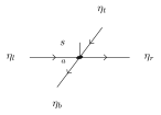
Then \(\rho _v^o(g)_{\sigma ,\eta } =\rho _\square (g)_{j_v\sigma ,j_v\eta }\). For coefficient vectors, let \(J_vx=x\circ j_v^{-1}\). The corresponding identities are \(J_v\rho _v^o(g)=\rho _\square (g)J_v\) and \(\mathcal A_v=\mathcal A J_v\). Hence \(G\)-injectivity of \(\mathcal A\) for \(\rho _\square \) implies \(G\)-injectivity of every \(\mathcal A_v\) for \(\rho _v^o\). In numbered virtual coordinates the local map is \(\mathcal A_vE_v\) and is \(G\)-injective for \(E_v^{-1}\rho _v^oE_v\).
The outgoing indices \(1,2\) contribute \(U_{g^{-1}}^T\); indices \(0,3\) contribute \(U_g\). Reindexing the four incidence factors gives (129). Reindexing the finite coefficient sum by \(j_v\) gives both intertwining identities. Since \(J_v\) is invertible, invariance and injectivity on invariant vectors pass from \(\mathcal A\) to \(\mathcal A_v\). Reindex once more by \(E_v\) to obtain the numbered assertion.
For every finite group representation \(U\) on a finite alphabet \(X\), there are a finite physical dimension \(p\) and a native tensor \(b:X^4\times \{ 0,\ldots ,p-1\} \to \mathbb {C}\) which is \(G\)-injective for \(\rho _\square \).
Let \(\Pi =|G|^{-1}\sum _g\rho _\square (g)\) and enumerate the coefficient basis of \(\mathbb {C}^{X^4}\) by a linear isomorphism \(E\) to \(\mathbb {C}^p\), with \(p=|X|^4\). Take \(b\) to be the matrix entries of \(E\Pi \). The average satisfies \(\Pi \rho _\square (g)=\Pi \) and is the identity on invariant vectors. Composing with \(E\) therefore gives the required invariance and restricted injectivity.
38.9.2 Commuting closures satisfy the original plaquette constraints
On any finite simple graph, let \(a_v\) be arbitrary site tensors with finite virtual alphabet \(X\), and insert a matrix \(K_e\) on each ordered bond. Suppose \(K_e=1\) whenever both endpoints lie in \(R\). For every fixed exterior physical configuration \(\tau \), the resulting vector \(\Psi _K(\, \cdot \, ,\tau )\) on \(R\) belongs to the original regional contraction range \(\operatorname {im}\mathcal C_R\). No invertibility, group symmetry, or positivity of the inserted matrices is required.
Split endpoint assignments into internal labels and pairs \(\zeta \) on all noninternal edges. The identity matrices on internal edges force their two endpoint labels to agree. For fixed \(\zeta \), the remaining coefficient is
Here \(\theta (\zeta )\) selects the retained endpoint on every crossing edge. Each summand is a boundary column of the original regional map, so the sum belongs to its range.
Let \(O^h_v\) act on the native rightward bond from \(v\), and \(O^v_v\) on the downward bond from \((x,y+1)\) to \(v=(x,y)\). For an ordered edge \(e=(t,h)\) put
Thus a transpose is inserted exactly when the native arrow and ordered-edge arrow disagree.
Reindex all native top/right/down/left labels by the incidence bijections \(j_v\), then regroup them into ordered endpoint pairs. The horizontal and vertical bond coefficients become, respectively,
Equations (134) and (137) give exactly these entries in both possible vertex orders. The site factors are unchanged, so the reindexed finite sums agree.
For \(v=(x,y)\) let \(R_v=v+\{ (0,0),(1,0),(1,1),(0,1)\} \). Place the horizontal closure seam at \(x+2\) and the vertical closure seam at \(y+2\). For any \(g,h\in G\), the corresponding inserted graph matrices are the identity on every edge internal to \(R_v\). This assertion includes \(m=3\) or \(n=3\).
The first coordinates in \(R_v\) are \(x,x+1\), whereas \(x+2\) differs from both modulo \(m\ge 3\). The analogous statement holds for \(y,y+1,y+2\) modulo \(n\). An internal rightward edge cannot end at the horizontal seam, and an internal upward edge cannot end at the vertical seam. Their insertion matrices are therefore \(1\); any transpose required by ordered coordinates leaves \(1\) unchanged.
Let \(U\) be any representation on finite \(X\), and suppose \(\mathcal A\rho _\square (k)=\mathcal A\) for every \(k\in G\). If \(gh=hg\), every physical slice of the native closure \(\lvert a;(g,h)\rangle \) on \(R_v\) lies in \(\operatorname {im}\mathcal C_{R_v}\). Consequently the closure belongs to the full plaquette parent space. If \(P_v\ge 0\) and \(\ker P_v=\operatorname {im}\mathcal C_{R_v}\), then every embedded \(P_v\) annihilates it, and so does \(H=\sum _v(P_v\otimes 1_{R_v^c})\). In particular,
This implication uses only local virtual invariance, without semi-regularity or \(G\)-injectivity.
Local invariance and \(gh=hg\) move both closure seams to \(x+2,y+2\) without changing the vector. Theorem 38.9.2.4 makes every internal insertion on \(R_v\) the identity. After the native-to-ordered contraction identity, formula (131) expresses each physical slice as a sum of unrestricted regional boundary columns. For the four-site plaquette, collecting equal boundary labels gives the contraction below. All four sites carry \(a\).
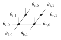
The coefficients \(c_\tau \) include the exterior contraction and every crossing insertion. Each local term therefore annihilates every closure slice. Summing the terms gives \(H\lvert a;(g,h)\rangle =0\); linearity proves (139).
38.9.3 Dimension and exhaustion of the full kernel
Let \(G\) be finite, let \(U\) be one unitary semi-regular representation on finite \(X\), and let \(a\) be one \(G\)-injective native tensor for \(\rho _\square \), repeated at every vertex of a torus with \(m,n\ge 3\). For each native plaquette \(R_v\), let \(P_v\ge 0\) have kernel \(\operatorname {im}\mathcal C_{R_v}\) and set \(H=\sum _v(P_v\otimes 1_{R_v^c})\). If \(\mathcal K_G=\{ (g,h)\in G^2:gh=hg\} /G\), with simultaneous conjugation, then
The block decomposition and its positive multiplicities are consequences of \(U\); no expansion of a parent vector into closures is assumed. This is the stated uniform-torus case of [ 272 , Theorem 5.9 ] .
Native incidence coordinates make every graph tensor \(G\)-injective for the rightward/downward orientation. The torus has degree four. Every vertex belongs to its plaquette, and every edge has both endpoints in a native plaquette. Theorem 38.8.2.5 therefore identifies the entire parent space of \(a\) with that of the oriented regular averaging tensor. Independently construct a native \(G\)-injective site \(b\) for the regular representation using Theorem 38.9.1.5. Fixed-representation comparison identifies its parent space with the same oriented regular canonical space. The already established regular native-torus theorem gives dimension \(|\mathcal K_G|\) for \(b\). Thus
Finally, positivity and the genuine local kernel conditions give \(\ker H=\mathcal P_{\{ R_v\} }(a)\).
Under the hypotheses of Theorem 38.9.3.1,
Thus the commuting closure vectors exhaust the entire positive plaquette-parent kernel for one repeated \(G\)-injective tensor and one uniform unitary semi-regular representation on native tori of periods at least three. This is the corresponding case of [ 272 , Theorems 5.7 and 5.9 ] .
Let \(\mathcal V\) be the span on the right of (142). Invariance gives \(\mathcal V\subseteq \ker H\) by (139). Closures in the same simultaneous-conjugacy class coincide, and semi-regular \(G\)-injectivity makes the vectors from distinct commuting classes linearly independent. Hence \(\dim \mathcal V=|\mathcal K_G|\) by Theorem 35.1.6.10. Equation (140) gives \(\dim \ker H=|\mathcal K_G|\). Inclusion and equal finite dimension imply \(\mathcal V=\ker H\). Taking canonical positive plaquette interactions identifies the same span with the full intersection of regional range conditions.
38.9.4 Labelled bonds and the four cuts
Let \(w,\ell \ge 0\) and \(\Lambda =\mathbb Z_w\times \mathbb Z_\ell \). A bond is a pair \(e=(v,d)\) with \(d\in \{ \mathrm H,\mathrm V\} \). Its tail \(s(e)\) and head \(t(e)\) are
The direction is part of the bond label. At period two, the two bonds connecting the same vertices are distinct; at period one, the head and tail incidences of a loop are distinct.
Suppose \(w,\ell {\gt}0\). For \(c\in \mathbb Z_w\) and \(r\in \mathbb Z_\ell \), set
A cut endpoint is a pair \((e,\varepsilon )\) with \(e\in E_{c,r}\) and \(\varepsilon \in \{ -,+\} \), recording the tail or the head.
When \(w=\ell =2\), there are eight labelled bonds. Each \(E_{c,r}\) contains four bonds and has eight distinct endpoints. Every bond \(e=((x,y),d)\) is uncut in \(E_{x,y}\).
The bond set has \(2\cdot 2\cdot 2=8\) elements. For each of the four choices of \((c,r)\), exactly two horizontal and two vertical bonds satisfy (144). Each has two endpoints. A bond anchored at \((x,y)\) is outside \(E_{x,y}\) because \(x+1\ne x\) and \(y+1\ne y\) in \(\mathbb Z_2\).
For \(w,\ell {\gt}0\), the incidences at \(v=(x,y)\) are in bijection with \(\{ \mathrm H,\mathrm V\} \times \{ -,+\} \). The inverse bijection is
Thus every vertex has four incident endpoint indices, including when a period equals one.
38.9.5 Flat group labels on the bonds
For a group \(G\), an assignment \(p:E\to G\) has horizontal and vertical components \(a_{x,y}=p((x,y),\mathrm H)\) and \(b_{x,y}=p((x,y),\mathrm V)\). We write \(p=(a,b)\) for these components.
A vertex assignment \(q:\Lambda \to G\) acts by
Pointwise multiplication of vertex assignments satisfies \(1\cdot p=p\), \(q\cdot (r\cdot p)=(qr)\cdot p\), and \(q^{-1}\cdot (q\cdot p)=p\).
The assignment \(p=(a,b)\) is flat if every plaquette satisfies
For every \(q\), the assignment \(q\cdot p\) is flat if and only if \(p\) is flat.
Bond flatness of \((a,b)\) is equivalent to flatness of the rightward and upward bond labels \((a,b^{-1})\): \(b_{x+1,y}^{-1}a_{x,y}=a_{x,y+1}b_{x,y}^{-1}\).
Multiplying (147) on the left by \(b_{x+1,y}^{-1}\) and on the right by \(b_{x,y}^{-1}\) and reversing the resulting equality gives the rightward-upward condition, while multiplication by the inverse factors gives the converse.
For the group labels of the two closures in [ 272 , Theorem 5.5 and Definition 5.6 ] , given \(g,h\in G\), the standard closure assignment \(\kappa (g,h)\) is
The assignment \(\kappa (g,h)\) is flat if and only if \(gh=hg\).
The relative labels of \(q\) are \(q\cdot 1\), namely \(p_e=q_{t(e)}q_{s(e)}^{-1}\). They are flat, since the identity assignment is flat and vertex gauges preserve flatness.
Suppose \(w,\ell {\gt}0\). For \(0\le x{\lt}w\) and \(0\le y{\lt}\ell \), put \(A_x=a_{x-1,0}\cdots a_{0,0}\) and \(B_{x,y}=b_{x,y-1}^{-1}\cdots b_{x,0}^{-1}\), with empty products equal to \(1\). Define \(q_{x,y}=(B_{x,y}A_x)^{-1}\).
If \(p\) is flat, then the inverse rooted path product satisfies \(q\cdot p=\kappa (B_{0,\ell }^{-1},A_w)\).
Applying the two rooted-path identities of Theorem 35.1.4.150 to \((a,b^{-1})\) yields the claimed horizontal component directly, while inverting the vertical identity gives the downward component.
For every \(w,\ell {\gt}0\), a bond assignment is flat if and only if \(p=q\cdot \kappa (g,h)\) for some vertex assignment \(q\) and commuting \(g,h\). Equivalently, a flat assignment admits \(q\) with \(q\cdot p=\kappa (g,h)\). This includes periods one and two.
The based holonomies \(B_{0,\ell }\) and \(A_w\) commute, hence so do \(g=B_{0,\ell }^{-1}\) and \(h=A_w\). Theorem 38.9.5.10 gives \(q\cdot p=\kappa (g,h)\); applying \(q^{-1}\) gives the other form. Conversely, commuting closure labels are flat and remain flat under a vertex gauge.
Suppose \(G\) is finite and \(w,\ell {\gt}0\). For any function \(f\) on bond assignments with values in a commutative additive monoid, \(\sum _r f(r\cdot (q\cdot p))=\sum _r f(r\cdot p)\).
Substituting \(r\cdot (q\cdot p)=(rq)\cdot p\) and reindexing the sum by the bijection \(r\mapsto rq\) of vertex assignments gives the equality.
38.9.6 Moving the commuting seams
Define \(\kappa _{c,r}(g,h)\) by replacing \(x+1=0\) and \(y+1=0\) in (152) by \(x+1=c\) and \(y+1=r\). In particular, \(\kappa _{0,0}(g,h)=\kappa (g,h)\).
For \(w,\ell {\gt}0\), write \(s_{k,c}(x)=k^{-1}\) when the least nonnegative representatives satisfy \(x{\lt}c\), and \(s_{k,c}(x)=1\) otherwise. Set \(q_{c,r}(x,y)=s_{g^{-1},r}(y)s_{h,c}(x)\).
In the group-valued form of the string movement in [ 272 , Section 5 ] , if \(gh=hg\) and \(w,\ell {\gt}0\), then
In the first two lines, a one-coordinate function denotes its pullback to \(\Lambda \). The first line needs only \(w{\gt}0\) and the second only \(\ell {\gt}0\). The last line in particular gives a vertex gauge taking the standard closure to any chosen pair of seams.
The one-dimensional seam identity gives the changed horizontal component. Every value of \(s_{h,c}\) commutes with \(g\), so conjugation leaves the vertical component fixed. The inverse-label seam identity gives the vertical movement, while commutation fixes the horizontal component. Composing the horizontal gauge with the vertical gauge gives their pointwise product \(q_{c,r}\).
For finite \(G\), positive periods, commuting \(g,h\), and any function \(f\) into a commutative additive monoid, \(\sum _q f(q\cdot \kappa _{c,r}(g,h)) =\sum _q f(q\cdot \kappa (g,h))\).
Replacing \(\kappa _{c,r}(g,h)\) via (153) and reindexing the orbit sum by multiplication with \(q_{c,r}\) gives the equality.
On individual bonds, write \(\kappa _e(g,h)\) and \(\kappa _{c,r;e}(g,h)\) for the assignments whose horizontal and vertical components are \(\kappa (g,h)\) and \(\kappa _{c,r}(g,h)\).
If \(e\notin E_{c,r}\), then \(\kappa _{c,r;e}(g,h)=1\).
In each direction, being outside the cut makes the seam condition false.
For positive periods and commuting \(g,h\), there exists \(q:\Lambda \to G\) such that \(q_{t(e)}\kappa _e(g,h)q_{s(e)}^{-1} =\kappa _{c,r;e}(g,h)\) for every bond \(e\).
Taking the gauge of Theorem 38.9.6.3 and reading its horizontal or vertical equality according to the direction of \(e\) gives the bondwise identity.
For positive periods, every flat assignment \(p:E\to G\) admits a vertex assignment \(q\) and commuting \(g,h\) with \(q_{t(e)}p_eq_{s(e)}^{-1}=\kappa _e(g,h)\) for every \(e\).
Classifying the horizontal and vertical components and evaluating the resulting pair of equalities in the direction of each bond gives the claim.
Let \(w=\ell =2\). Suppose \(p_e=q_{t(e)}q_{s(e)}^{-1}\) for every \(e\notin E_{c,r}\). Then \(b_{c+1,r}a_{c,r+1}=a_{c,r}b_{c,r}\).
The four bonds in this equality are uncut. Substitution gives
38.9.7 Contractions with independently sized bonds
Let \(\mathcal V\) and \(\mathcal E\) be finite sets of vertices and labelled oriented bonds, with tail and head maps \(t,h:\mathcal E\to \mathcal V\). Each bond \(e\) has its own finite alphabet \(X_e\), and each vertex \(v\) has its own physical alphabet \(Y_v\). Parallel bonds remain distinct; a bond with \(t(e)=h(e)\) has two distinct incidences. These conventions express the linkwise matching in [ 272 , Definition 5.1 ] .
The incidence set is \(\mathcal E\times \{ -,+\} \), where \(-\) is the tail and \(+\) the head. Put \(I_v=\{ (e,\epsilon ):v(e,\epsilon )=v\} \) and \(\mathcal X_v=\prod _{(e,\epsilon )\in I_v}X_e\). An incidence configuration \(\beta \) assigns \(\beta _{e,\epsilon }\in X_e\) independently. Restriction to \(I_v\) defines a bijection \(R:\prod _{e,\epsilon }X_e\to \prod _v\mathcal X_v\) with \((R\beta )_v(e,\epsilon )=\beta _{e,\epsilon }\); its inverse reads the coordinate in the unique incident vertex. The bond-pair bijection is \(S\beta =(\beta _{e,+},\beta _{e,-})_{e\in \mathcal E}\).
For factors in any commutative monoid, \(\prod _v\prod _{p\in I_v}f(p)=\prod _p f(p) =\prod _e f(e,-)f(e,+)\). For functions \(f_e:X_e^2\to R\) into a commutative semiring,
The sets \(I_v\) partition the incidence set. Regroup first by this partition and then by the two signs of each bond. For the sum, change coordinates by \(S\) and apply finite distributivity.
Let \(A_v(\eta ,s)\) be the coefficient of a tensor with virtual configuration \(\eta \in \mathcal X_v\) and physical index \(s\in Y_v\). For matrices \(B_e\in \operatorname {Mat}_{X_e}(\mathbb {C})\) define \(w_B(\beta )=\prod _e B_e(\beta _{e,+},\beta _{e,-})\) and
Thus every matrix has its head index as row and tail index as column. The second expression is the change of coordinates by \(R\).
For \(C\subseteq \mathcal E\), let \(\partial C=C\times \{ -,+\} \) and \(\mathcal X_{\partial C}=\prod _{(e,\epsilon )\in \partial C}X_e\). Write \(r_C\beta =\beta |_{\partial C}\) and \(w_C(\beta )=\prod _{e\notin C}\delta _{\beta _{e,+},\beta _{e,-}}\). The linear cut map is
Its range is \(\mathcal S_{A,C}=\operatorname {im}\mathcal C_{A,C}\). Equivalently, \(\psi \in \mathcal S_{A,C}\) if and only if one \(M\) satisfies \(\mathcal C_{A,C}(M)(\sigma )=\psi (\sigma )\) for every \(\sigma \). The function \(M\) may correlate all cut indices.
Let \(\delta _\eta \) denote a coordinate vector on \(\mathcal X_{\partial C}\). Then
A matrix family determines the particular boundary \(M_B(\eta )=\prod _{e\in C}B_e(\eta _{e,+},\eta _{e,-})\). Its value at \(r_C\beta \) is the product of these same cut-bond factors, and \(\mathcal C_{A,C}(M_B)=\mathcal N_A(B^C)\), where \(B^C_e=B_e\) on \(C\) and \(B^C_e=I\) elsewhere. Define \(E^\eta _e\) to be the matrix unit \(|\eta _{e,+}\rangle \langle \eta _{e,-}|\) on \(C\), and \(I\) elsewhere. Then \(M_{E^\eta }=\delta _\eta \) and \(\mathcal C_{A,C}(\delta _\eta )=\mathcal N_A(E^\eta )\).
Expand \(M=\sum _\eta M(\eta )\delta _\eta \) and use linearity. In the contraction with \(M_B\), the factors on \(C\) are the entries of \(B_e\), and the remaining factors are identity entries. Products of matrix-unit entries equal one exactly when all cut coordinates equal \(\eta \), proving the last assertions without factoring a general \(M\).
For finite input alphabets \(J_v\), arbitrary output alphabets \(K_v\), and matrices \(F_v: \mathbb {C}^{J_v}\to \mathbb {C}^{K_v}\), put \((\bigotimes _v F_v)_{\tau ,\sigma }=\prod _v F_v(\tau _v,\sigma _v)\). The associated linear map \(\mathcal F\) satisfies
Products compose coordinatewise: \((\bigotimes _vF_v)(\bigotimes _vL_v) =\bigotimes _v(F_vL_v)\), at both the matrix and linear-map levels. Products of identities are identities. The product with \(P_v\) at one coordinate and identities elsewhere acts by \(\psi (\tau )\mapsto \sum _sP_v(\tau _v,s)\psi (\tau [v\leftarrow s])\). If each \(P_v\) fixes every slice \(s\mapsto \psi (\tau [v\leftarrow s])\), then \(\bigotimes _vP_v\) fixes \(\psi \); the \(P_v\) need not be projections.
Finite distributivity separates the intermediate sum in a matrix product into one sum at each coordinate. Identity entries force equality of the remaining coordinates. For the fixed-vector assertion, induct on the finite set of coordinates at which \(P_v\) replaces the identity, using the one-coordinate formula and coordinatewise composition.
Every one-coordinate slice of \(\mathcal F\chi \) lies in \(\operatorname {im}F_v\). If all input and output alphabets are finite, the converse holds:
Empty alphabets, an empty vertex set, zero matrices, and different local ranks are allowed.
For the forward implication, expand a slice as a sum of columns of \(F_v\), with coefficients obtained by contracting all other coordinates. For each \(v\), choose a linear right inverse on \(\operatorname {im}F_v\) and extend it to a map \(L_v\) on the output space. Thus \(F_vL_v\) fixes every slice. The preceding theorem gives \((\bigotimes _vF_vL_v)\psi =\psi \), so \((\bigotimes _vL_v)\psi \) is a preimage.
38.9.8 Matched representations and a common local inverse
Retain the incidence coordinates of Definition 38.9.7.1. Following the matching convention of [ 272 , Definition 5.1 ] , let \(G\) be a finite group and let each bond carry a representation \(U_e:G\to \operatorname {GL}(\mathbb {C}^{X_e})\), with the same \(U_e\) occurring at both ends of that bond and the dual action at its tail.
The representation \(\rho _v\) acts by the matrix
It satisfies \(W_v(1)=I\) and \(W_v(gh)=W_v(g)W_v(h)\), so \(\rho _v(g)x=W_v(g)x\). The local coefficient map is \(T_vx(s)=\sum _{\eta \in \mathcal X_v}A_v(\eta ,s)x(\eta )\). The identity and multiplication laws follow coordinatewise, since \(g\mapsto U_e(g^{-1})^{\mathsf T}\) is also a representation.
For any representation \(\rho _v\) on \(\mathbb {C}^{\mathcal X_v}\), let \(P_v=|G|^{-1}\sum _g\rho _v(g)\) and define \(A_v^0(\eta ,s)=(P_v)_{s,\eta }\). Its local coefficient map is exactly \(P_v\). For the incident representation, \(A_v^0(\eta ,s)=|G|^{-1}\sum _gW_v(g)_{s,\eta }\).
Every \(A_v^0\) is \(G\)-injective for its representation \(\rho _v\). In particular this holds for independently chosen incident bond actions.
Right multiplication by \(\rho _v(g)\) permutes the group average, so \(P_v\rho _v(g)=P_v\). On the invariant subspace \(P_v\) is the identity, hence is injective there.
Local sums expand independently, and local scalars multiply: \(\mathcal N_{\sum _i A^i}(B)=\sum _{q:\mathcal V\to J} \mathcal N_{(A^{q_v}_v)_v}(B)\) and \(\mathcal N_{(c_vA_v)_v}(B)=(\prod _vc_v)\mathcal N_A(B)\). For fixed vertex labels \(q\), contracting the local matrices \(W_v(q_v)\) gives the product of the entries of \(U_e(q_{h(e)})B_eU_e(q_{t(e)}^{-1})\). Consequently, with \(n=|\mathcal V|\),
No semi-regularity or unitarity is required in this independent-bond version of the projector contraction of [ 272 , Theorem 5.9 ] .
Expanding each local average collects the factor \(|G|^{-n}\), and regrouping the incident matrix factors by bonds turns the independent sum over the two indices of each bond into the displayed three-matrix product by (155).
As in the virtual symmetry of [ 272 , Definition 5.1 ] , for any \(q:\mathcal V\to G\) and arbitrary matrices \(B_e\), set \(B_e^q=U_e(q_{h(e)})B_eU_e(q_{t(e)}^{-1})\). Then \(\mathcal N_{A^0}(B^q)=\mathcal N_{A^0}(B)\); in particular, the group-label change \(p_e\mapsto q_{h(e)}p_eq_{t(e)}^{-1}\) preserves the canonical network.
Changing the vertex summation variable from \(r\) to \(rq\) in (162), the inverse at a tail reverses the product in precisely the required order.
Given finite \(Y_v\) and matrices \(F_v:\mathbb {C}^{Y_v}\to \mathbb {C}^{Z_v}\), define \((FA)_v(\eta ,s)=\sum _tF_v(s,t)A_v(\eta ,t)\). Its local coefficient map is \(F_vT_v\). Equality of local coefficient maps at every site implies equality of tensor families, by evaluating those maps on every coordinate vector.
Let \(\mathcal F=\bigotimes _vF_v\). For every joint boundary \(M\) and every bond-matrix family \(B\), \(\mathcal F\mathcal C_{A,C}(M)=\mathcal C_{FA,C}(M)\) and \(\mathcal F\mathcal N_A(B)=\mathcal N_{FA}(B)\).
Expanding the product physical map, interchanging the finite physical and incidence sums, and distributing the product of the local sums leaves the factors \(M(r_C\beta )w_C(\beta )\) and \(w_B(\beta )\) unchanged.
Suppose the physical alphabets are finite and every \(T_v\) is \(G\)-injective for a representation \(\rho _v\) on its virtual space. There are \(L_v\) with \(L_vT_v=P_v\); hence \(LA=A^0\). Invariance alone gives \(T_vP_v=T_v\) and \(TA^0=A\). Put \(\mathcal L=\bigotimes _vL_v\) and \(\mathcal T=\bigotimes _vT_v\). For every cut \(C\) and every joint boundary \(M\),
Therefore, for any nonempty family \((C_i)_{i\in J}\) of cuts,
Each \(L_v\) is given by the left-inverse characterization of \(G\)-injectivity, and averaging the invariance equations gives \(T_vP_v=T_v\), so the physical-contraction identities yield (163) with the same \(M\). If \(\psi \) lies in every original cut range, then \(\mathcal L\psi \) lies in every canonical range, and choosing one cut in the nonempty family gives \(\mathcal T\mathcal L\psi =\psi \); conversely, \(\mathcal T\) carries each canonical range into the corresponding original range.
The identity tensor has coefficients \(I_v(\eta ,s)=\delta _{\eta ,s}\), so \(\mathcal N_I(B)(\sigma )=w_B(R^{-1}\sigma )\). Define the product invariant projection \(\mathcal P=\bigotimes _vP_v\).
For any representations \(\rho _v\), any joint cut boundary \(M\), and any matrices \(B_e\), \(\mathcal P\mathcal C_{A^0,C}(M)=\mathcal C_{A^0,C}(M)\) and \(\mathcal P\mathcal N_I(B)=\mathcal N_{A^0}(B)\).
Canonical recovery applied to the \(G\)-injective tensors \(A^0\) gives the first equality; for the second, applying \(P_v\) to the physical leg of \(I_v\) gives \(A_v^0\), and commuting these local changes through the network completes the proof.
38.9.9 Coherent coefficients forced by complementary cuts
Retaining the independent incidence spaces and incident representations of Definitions 38.9.7.1 and 38.9.8.1, this section derives a bond-product expansion from cut membership before extracting its coefficients via the trace duality of [ 272 , Lemma 4.6 ] , as used in the four-block comparison of [ 272 , Theorem 5.5 ] .
The bijection \(J=SR^{-1}\) sends a site configuration to its head–tail bond pairs. It induces the coefficient permutation \((\mathcal R\psi )(\beta )=\psi (J^{-1}\beta )\). For a matrix family \(B\), let \(b_B(\sigma )=\prod _eB_e((J\sigma )_e^+,(J\sigma )_e^-)\), so \((\mathcal Rb_B)(\beta )=\prod _eB_e(\beta _e^+,\beta _e^-)\). For group labels \(p:\mathcal E\to G\), abbreviate \(b_p=b_{(U_e(p_e))_e}\).
Given linear functionals \(K_e\) on the bond matrices, define
With the source’s trace-dual functionals \(\ell _{e,g}(B)=\operatorname{tr}[U_e(g^{-1})B\Delta _e]\), write \(c_p(\psi )=(\bigotimes _e\ell _{e,p_e})(\psi )\) for this product functional.
For arbitrary \(K_e\) and \(B_e\), \(K(b_B)=\prod _eK_e(B_e)\). If every \(U_e\) is semi-regular, then
Thus two coherent sums in the \(b_p\) are equal if and only if their complete coefficient functions are equal.
Distributing (165) over the bond pairs evaluates the \(e\)-th sum as \(K_e(B_e)\) by expansion in matrix units. Trace duality then gives \(\ell _{e,p_e}(U_e(q_e))=\delta _{p_e,q_e}\), whose product is \(\delta _{p,q}\), and applying linearity to the entire coherent sum identifies each coefficient.
Let \(F_e:\mathbb {C}^G\to \mathbb {C}^{X_e\times X_e}\) have columns \(F_e((a,b),g)=U_e(g)_{a,b}\). Each representation matrix is therefore a vector in \(\operatorname {im}F_e\). The slice at bond \(e\) and remaining configuration \(\tau \) is \(S_{e,\tau }\psi (s)=(\mathcal R\psi )(\tau [e\leftarrow s])\). Put \(B_e(q)=U_e(q_{h(e)})B_eU_e(q_{t(e)}^{-1})\).
A coordinate slice of \(\prod _w f_w(\tau _w)\) is \((\prod _{w\ne e}f_w(\tau _w))f_e\). With \(n=|\mathcal V|\), the canonical contraction and its regrouping obey
These identities require neither semi-regularity nor restrictions on \(B\).
Separating the \(e\)-th factor establishes the slice identity, while regrouping (162) by \(J\) yields the first two formulas and applying the product-functional identity to each term gives the third.
If \(B_e=I\), then every \(S_{e,\tau }\mathcal N_{A^0}(B)\) lies in \(\operatorname {im}F_e\). Consequently, if \(e\notin C\) and \(\psi \in \mathcal S_{A^0,C}\), then \(S_{e,\tau }\psi \in \operatorname {im}F_e\) for every \(\tau \), even when the cut boundary is arbitrarily correlated.
In a summand of (167), an identity insertion gives \(B_e(q)=U_e(q_{h(e)}q_{t(e)}^{-1})\), so every slice is a scalar multiple of this representation matrix and sums retain membership in \(\operatorname {im}F_e\). Expanding a general boundary into fixed configurations produces matrix-unit networks that still have \(B_e=I\) when \(e\notin C\).
Let \((C_i)_{i\in J}\) be any family of cuts such that every bond is uncut in at least one \(C_i\). If \(\psi \in \mathcal S_{A^0,C_i}\) for every \(i\), then \(\mathcal R\psi \in \operatorname {im}(\bigotimes _eF_e)\). In particular there are coefficients \(a_p\) with \(\psi =\sum _pa_pb_p\). If all \(U_e\) are semi-regular, this becomes
Choosing a cut for each bond that leaves it uncut, the preceding theorem places every slice in \(\operatorname {im}F_e\). The product-range criterion then provides a preimage under \(\bigotimes _eF_e\) whose entries are the coefficients \(a_p\), and applying \(c_p\) to the whole expansion identifies \(a_p=c_p(\psi )\) in the semi-regular case.
Assume every \(U_e\) is semi-regular. If \(B_e=I\) outside \(C\) and no \(q:\mathcal V\to G\) satisfies \(p_e=q_{h(e)}q_{t(e)}^{-1}\) simultaneously for all \(e\notin C\), then \(c_p(\mathcal N_{A^0}(B))=0\). The same vanishing holds for every \(\psi \in \mathcal S_{A^0,C}\). Equivalently,
For any vertex assignment \(q\) in the extracted sum of (167), incompatibility yields an uncut bond with \(p_e\ne q_{h(e)}q_{t(e)}^{-1}\) whose trace-dual factor is zero, so every summand vanishes. Expanding an arbitrary boundary into fixed-coordinate columns and using their matrix-unit realization extends this vanishing, whose contrapositive is the stated implication.
38.9.10 The four-block closure property
The four blocks in [ 272 , Theorem 5.5 ] occupy \(\Lambda =(\mathbb Z/2\mathbb Z)^2\). There are eight labelled bonds, including two distinct bonds between each horizontal or vertical pair of blocks. Every bond \(e\) has its own finite virtual alphabet \(X_e\) and semi-regular representation \(U_e\); every block has its own finite physical alphabet \(Y_v\). The head acts by \(U_e\) and the tail by \(U_e^{-\mathsf T}\), so the two incident tensors use the same representation on their shared bond.
Let \(C_{c,r}\) be the cut consisting of horizontal bonds with head column \(c\) and vertical bonds with tail row \(r\). Its virtual domain is \(\mathcal X_{\partial C_{c,r}}\), with eight independent incidence indices. Define
Here \(p^{g,h}\) is \(h\) on the horizontal seam, \(g\) on the vertical seam, and \(1\) elsewhere. Membership in \(\mathcal I_A\) means membership in all four displayed ranges. Every bond is uncut for at least one of these four choices: its own base-vertex cut leaves it uncut.
Let \(G\) be finite. Assign a semi-regular representation \(U_e\) to each of the eight bonds, and let the four tensors \(A_v\) be \(G\)-injective for their incident representations. Then
In this form of [ 272 , Theorem 5.5 ] , the bond and physical dimensions may differ independently, each boundary \(M\) is an arbitrary tensor on all eight open incidences, and algebraic semi-regularity suffices (containing the unitary convention of the source as a special case).
Write \(A^0\) for the four incident averaging tensors and \(\mathcal T=\bigotimes _vT_v\) for the product of the original local coefficient maps. A common product of genuine \(G\)-injective inverses gives \(\mathcal I_A=\mathcal T(\mathcal I_{A^0})\); the same physical map gives \(\mathcal T(\mathcal Z_{A^0})=\mathcal Z_A\). For the canonical tensors, every commuting seam can be moved to any of the four cuts, giving explicit boundary tensors. Conversely, uncut-bond slices give a coherent expansion of every \(\psi \in \mathcal I_{A^0}\). Trace-dual extraction forces each nonzero coefficient to satisfy every plaquette equation. A vertex gauge sends every such flat assignment to commuting seams, and the product invariant projection turns each bare bond product into its closure. Hence \(\mathcal I_{A^0}=\mathcal Z_{A^0}\), proving the result.
For arbitrary local physical maps and \(\mathcal F=\bigotimes _vF_v\), \(\mathcal F\zeta _A(g,h)=\zeta _{FA}(g,h)\) and \(\mathcal F(\mathcal Z_A)=\mathcal Z_{FA}\). For \(G\)-injective \(A\), let \(\mathcal T=\bigotimes _vT_v\) and let \(A^0\) be the incident averaging tensors. Then \(\mathcal I_A=\mathcal T(\mathcal I_{A^0})\). Invariance of \(A\) alone gives \(\mathcal T(\mathcal Z_{A^0})=\mathcal Z_A\).
Commuting physical maps through the network defining \(\zeta _A\) and taking spans gives the first two identities. Applying (164) to the four cuts with \((0,0)\) chosen in this nonempty family gives \(\mathcal I_A=\mathcal T(\mathcal I_{A^0})\), and \(T_vP_v=T_v\) identifies the recovered tensors with \(A_v\) themselves.
On the four-block torus, the canonical tensors are \(A_v^0(\eta ,s)=(P_v)_{s,\eta }\) and their product projection is \(\mathcal P=\bigotimes _{v\in \Lambda }P_v\). The physical alphabet of the canonical tensor at \(v\) is precisely its own \(\mathcal X_v\).
If \(gh=hg\), then \(\zeta _{A^0}(g,h)\in \mathcal S_{A^0,C_{c,r}}\) for every \((c,r)\). In particular \(\mathcal Z_{A^0}\subseteq \mathcal I_{A^0}\). This inclusion requires no semi-regularity.
Moving the seams to \((c,r)\) by the group-valued vertex gauge produces labels \(p^{g,h;c,r}\) equal to \(1\) off \(C_{c,r}\). For the explicit boundary \(M(\eta )=\prod _{e\in C_{c,r}} U_e(p^{g,h;c,r}_e)_{\eta _{e,+},\eta _{e,-}}\), the matrix-boundary contraction and vertex-gauge invariance identify its image with \(\zeta _{A^0}(g,h)\); taking spans and intersecting the four ranges gives the inclusion.
For every bond assignment \(p\), one has \(\mathcal P b_p=\mathcal N_{A^0}((U_e(p_e))_e)\). If \(p\) is flat, there exist \(g,h\) with \(gh=hg\) and \(\mathcal P b_p=\zeta _{A^0}(g,h)\); thus \(\mathcal P b_p\in \mathcal Z_{A^0}\).
The bare product \(b_p\) is the identity-site network, so product averaging proves the first equality. Flat labelled bonds are vertex-gauge equivalent to two commuting seams. Canonical vertex-gauge invariance therefore gives the asserted closure.
Suppose every \(U_e\) is semi-regular. If \(\psi \in \mathcal I_{A^0}\) and \(p\) is not flat, then \(c_p(\psi )=0\).
On the cut corresponding to a plaquette where flatness fails, \(c_p(\psi )\ne 0\) and (169) would give one vertex assignment realizing all four uncut labels simultaneously, whose relative labels would satisfy that plaquette equation.
If all eight bond representations are semi-regular, then \(\mathcal I_{A^0}\subseteq \mathcal Z_{A^0}\) and in fact \(\mathcal I_{A^0}=\mathcal Z_{A^0}\).
Let \(\psi \in \mathcal I_{A^0}\). Membership in the \((0,0)\) cut gives \(\mathcal P\psi =\psi \). Every bond is uncut in at least one of the four cuts, so (168) and linearity give
Nonflat terms vanish by coefficient extraction; each remaining projected term is a commuting closure. The forward inclusion proves equality.
38.9.11 Independent four-block closure classes
Retain the four blocks, eight separately represented bonds, and cut spaces of Definition 38.9.10.1. Write \(p^{g,h}\) for the standard seam labels and \(A^0\) for the four incident averaging tensors. Let \(K\) be the number of simultaneous conjugacy classes of commuting pairs in \(G\). The independence argument of [ 272 , Theorem 5.9 ] gives an exact dimension for this four-block intersection. The identification with a microscopic parent kernel is a separate geometric assertion.
For any \(x,g,h\in G\), one has \(p^{xgx^{-1},xhx^{-1}}_e=xp^{g,h}_ex^{-1}\) on every bond. Given pairs \((a,b),(g,h)\) and vertex labels \(q\), the identities
hold on all eight bonds if and only if \(q\) is constant, with value \(x=q_{(0,0)}\), and \(a=xgx^{-1}\) and \(b=xhx^{-1}\). Commutation is unnecessary here.
Both standard closures equal \(1\) off their seams. On those bonds the asserted identities give equality of neighboring vertex labels. Nonseam connectivity implies \(q_v=q_{(0,0)}\) at all four vertices. Reading the vertical bond based at \((0,-1)\) and the horizontal bond based at \((-1,0)\) gives \(a=xgx^{-1}\) and \(b=xhx^{-1}\). Conversely, these equalities give the seam identities, while constant conjugation fixes the identity labels on the other bonds.
Suppose \(G\) is finite and every \(U_e\) is semi-regular. Let \(E_{a,b}=c_{p^{a,b}}\) be the product of the eight bond trace-dual functionals. Then
Here \(C_G(g,h)=\{ x\in G:xg=gx,\ xh=hx\} \) is the common centralizer. In particular, the coefficient is zero for different simultaneous conjugacy classes. These formulas hold even for noncommuting pairs.
Expanding the four normalized local averages and applying the eight trace-dual functionals gives
Theorem 38.9.11.1 identifies the surviving labels with constant functions \(q_v=x\), proving (175). On the diagonal the surviving \(x\) are precisely the common centralizer. It contains the identity, so (176) is nonzero.
For a finite group and locally invariant tensors \(A_v\), one has \(\zeta _A(xgx^{-1},xhx^{-1})=\zeta _A(g,h)\) for all \(x,g,h\). Thus closures depend only on their simultaneous conjugacy class. Neither semi-regularity nor injectivity is needed for this assertion.
A constant vertex gauge transforms the two canonical seam labels by simultaneous conjugation and leaves the canonical network unchanged. Writing \(T_v\) for the original site maps, local invariance gives \(T_vP_v=T_v\). Hence \(\zeta _A(g,h)=(\bigotimes _vT_v)\zeta _{A^0}(g,h)\), which carries the equality to the original physical tensors.
For a simultaneous conjugacy class \(C=[(g,h)]\), define \(\zeta _A(C)=\zeta _A(g,h)\). This does not depend on the representative. The set of closures indexed by commuting pairs equals the set indexed by commuting pair-conjugacy classes.
Suppose each of the eight bond representations is semi-regular and every physical tensor is \(G\)-injective for its own incident action. Then the vectors \(\zeta _A(C)\) are linearly independent as \(C\) ranges over all pair-conjugacy classes. In particular, the commuting classes give a linearly independent family. The four physical alphabets and all eight virtual alphabets may differ independently.
First take the canonical tensors. Apply \(E_{g,h}\), for a representative of any fixed class \(C\), to a relation \(\sum _{C'}\lambda _{C'} \zeta _{A^0}(C')=0\). The off-class coefficients vanish, and the remaining equation is \(\lambda _C|G|^{-4}|C_G(g,h)|=0\). Thus every \(\lambda _C=0\). For the physical tensors, choose their genuine local inverses with \(L_vT_v=P_v\). Physical contraction gives \((\bigotimes _vL_v)\zeta _A(C)=\zeta _{A^0}(C)\) for every class \(C\). Applying this same linear map to a relation proves the result for \(A\). The inverse and scalar extraction are depicted below. Each vertical leg denotes a complete configuration, retaining its independently typed component indices; \(\mathcal L=\bigotimes _vL_v\).
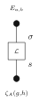 \(=\)
 \(\displaystyle =|G|^{-4} \sum _{x\in G}\mathbf1_{a=xgx^{-1},\, b=xhx^{-1}}\).
Under the hypotheses of Theorem 38.9.11.5, the commuting class-labelled closures form a basis of \(\mathcal I_A=\mathcal Z_A\). Both spaces have complex dimension \(K\), the number of simultaneous conjugacy classes of commuting pairs in \(G\).
The four-cut closure theorem gives \(\mathcal I_A=\mathcal Z_A=\operatorname{span}_{\mathbb {C}}\{ \zeta _A(C):C\text{ commuting}\} \). The stated family is linearly independent, so the dimension of its span is its cardinality \(K\).
The four boundary contractions.
Put \(A=(0,1)\), \(B=(1,1)\), \(C=(0,0)\) and \(D=(1,0)\). Write \(H_{xy}=((x,y),\mathrm H)\) and \(V_{xy}=((x,y),\mathrm V)\). The four contractions in [ 272 , Theorem 5.5 ] are \(\alpha (M)=\mathcal C_{0,0}(M)\), \(\beta (N)=\mathcal C_{1,0}(N)\), \(\gamma (P)=\mathcal C_{0,1}(P)\) and \(\delta (Q)=\mathcal C_{1,1}(Q)\). Each central tensor below is one arbitrary joint tensor on eight endpoints; the four outer wires are the four uncut identity pairings. A superscript \(+\) identifies a head endpoint, and \(-\) a tail endpoint. Thus two wires bearing the same bond label but different superscripts are independent arguments of the boundary tensor, not an identity pairing. The uncontracted physical legs are \(i_A,i_B,i_C,i_D\). The drawings move the boundary tensor to the centre without changing any incidence. Their displayed geometry does not identify parallel bonds.
\(\alpha (M)=\mathcal C_{0,0}(M)\).
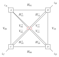
\(\beta (N)=\mathcal C_{1,0}(N)\).
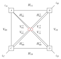
\(\gamma (P)=\mathcal C_{0,1}(P)\).
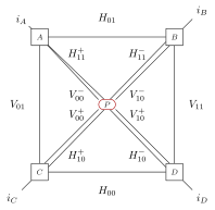
\(\delta (Q)=\mathcal C_{1,1}(Q)\).
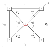
38.9.12 Four cut spaces with common coordinate alphabets
The following constructions give the common-coordinate specialization of the four boundary spaces in [ 272 , Theorem 5.5 ] , whose full statement is Theorem 38.9.10.2. Let \(X=\mathbb {Z}/w\mathbb {Z}\times \mathbb {Z}/\ell \mathbb {Z}\), where \(w,\ell {\gt}0\), and write \(e=(1,0)\) and \(n=(0,1)\). Horizontal bonds run from \(v\) to \(v+e\); vertical bonds run from \(v+n\) to \(v\). Let \(V\) be a finite virtual alphabet and \(P\) a physical alphabet. All eight bonds remain distinct when \(w=\ell =2\). Write \(\mathcal N_A(O^{\mathrm h},O^{\mathrm v})\) for the physical vector obtained from the bond contraction of Definition 35.1.4.1, with independent site tensors \(A_v:V^4\times P\to \mathbb {C}\).
The boundary configurations for the cut \((c,r)\) form \(\mathcal E=(V\times V)^{\mathbb {Z}/\ell \mathbb {Z}}\times (V\times V)^{\mathbb {Z}/w\mathbb {Z}}\). Each pair is ordered tail, head. For independent bond-end labels \(\beta :X\to V^4\), put
For an arbitrary joint boundary tensor \(M:\mathcal E\to \mathbb {C}\), define the linear map \(\mathcal C^A_{c,r}\) by
Put \(\mathcal S^A_{c,r}=\operatorname {ran}\mathcal C^A_{c,r}\). Thus \(\psi \in \mathcal S^A_{c,r}\) precisely when some \(M\) satisfies \((\mathcal C^A_{c,r}M)(\sigma )=\psi (\sigma )\) for every \(\sigma \). On \(X=(\mathbb {Z}/2\mathbb {Z})^2\), put \(\mathcal S^A=\bigcap _{c,r}\mathcal S^A_{c,r}\); membership means that each cut admits such a boundary tensor, which may depend on the cut. Here \(|\mathcal E|=|V|^8\).
The boundary occurs linearly in (183). The range descriptions follow by equality of all coefficients, and the intersection description follows by imposing all four range conditions. The two rows and two columns each contribute two independent endpoints, giving \(|V|^{2\cdot 2+2\cdot 2}=|V|^8\) configurations.
For bond matrices \(O^{\mathrm h}_v,O^{\mathrm v}_v\), define
Its value at \(R_{c,r}(\beta )\) is the product of the corresponding \(O^{\mathrm h}_v(\beta _v^2,\beta _v^1)\) and \(O^{\mathrm v}_v(\beta _v^4,\beta _v^3)\) on cut bonds, with factor one on every other bond. For fixed \(\eta \in \mathcal E\), let \(E^{\mathrm h}_{\eta ,v}=E_{\eta ^{\mathrm h,2}_{v_y}, \eta ^{\mathrm h,1}_{v_y}}\) and \(E^{\mathrm v}_{\eta ,v}=E_{\eta ^{\mathrm v,2}_{v_x}, \eta ^{\mathrm v,1}_{v_x}}\) be matrix units. Then \(M^{E_\eta }_{c,r}(\theta )=\delta _{\eta ,\theta }\).
Substitution of (178) selects the designated seam bonds. Every matrix unit fixes its two endpoints; their product is one exactly when all endpoint labels agree with \(\eta \).
Write \(\widehat O^{\mathrm h,c}_v=O^{\mathrm h}_v\) on \(v_x+1=c\) and \(\mathbb {1}\) elsewhere, and define \(\widehat O^{\mathrm v,r}\) analogously. Then
In particular, \(\mathcal C^A_{c,r}\delta _\eta \) is the network with \(E^{\mathrm h}_{\eta ,v}\) and \(E^{\mathrm v}_{\eta ,v}\) on cut bonds and identities elsewhere.
Multiplying the restricted product boundary by \(W_{c,r}\) gives the bond weights in (185), and expanding \(M=\sum _\eta M(\eta )\delta _\eta \) by linearity gives the second identity. Each fixed-boundary vector already belongs to the range, proving the reverse span inclusion, and the matrix-unit identity gives the final assertion.
Following the matching convention of [ 272 , Definition 5.1 ] , in which each link carries its own representation used at both ends, let \(G\) be a group and assign representations \(U^{\mathrm h}_v\) and \(U^{\mathrm v}_v\) on \(\mathbb {C}^V\) to the individual bonds. Their action on the top, right, down, left coordinates of site \(v\) is
The coefficient action is multiplication by this matrix. The bond family is unitary when every \(U^d_v(k)\) is unitary, and, for finite \(G\), is semi-regular when every individual representation \(U^d_v\) is semi-regular. These are separate conditions. For any representation \(\rho \) on \(\mathbb {C}^{V^4}\) of finite \(G\), put \(\Pi _\rho =|G|^{-1}\sum _k\rho (k)\) and \(A^0_\rho (t,r,b,l;s)=(\Pi _\rho )_{s,(t,r,b,l)}\). Its site map is \(\Pi _\rho \). Write \(A^0_v=A^0_{\rho _v}\) for the matched family; constant bond representations recover the uniform four-leg action and its averaging tensor.
The inverse transpose reverses the order twice, so (186) is a representation. The stated coefficient action and the site map of \(A^0_\rho \) follow by reading their matrix entries, and constant bond families give the uniform formulas by substitution.
For \(g,h\in G\), define
When every bond representation is \(U\), these are the site-dependent uniform closures and their span. If also every site tensor equals \(A\), the closure is \(\mathcal M(A\mid g,h)\) of Definition 35.1.4.96.
Suppose every bond carries \(U\) and each site map obeys \(\mathcal P(A_v)\rho (k)=\mathcal P(A_v)\) for every \(k\in G\). If \(gh=hg\), then for every cut \((c,r)\),
Consequently \(\mathcal Z_A\subseteq \mathcal S^A\) on the two-by-two torus.
Setting \(B(t,r,b,l;(v,s))=A_v(t,r,b,l;s)\) with \((v,s)\) as its physical label preserves invariance separately at each physical label. Applying Theorem 35.1.4.99 to \(B\) and the configuration \(v\mapsto (v,\sigma _v)\) together with the product-boundary identity gives the explicit boundary tensor in (192), and taking spans proves the inclusion.
For \(x,c\in \mathbb {Z}/m\mathbb {Z}\), with \(m{\gt}0\), use representatives \(\bar x,\bar c\in \{ 0,\ldots ,m-1\} \) and put \(s_{k,c}(x)=k^{-1}\) if \(\bar x{\lt}\bar c\), and \(s_{k,c}(x)=1\) otherwise.
Write \(K^c_k(x)=k\) if \(x+1=c\), and \(K^c_k(x)=1\) otherwise. For every \(k\in G\),
If \(kl=lk\), then \(s_{k,c}(x)\) commutes with \(l\).
Checking the wrap \(x+1=0\), the crossing \(x+1=c\), and the two intervals between them shows that adjacent factors cancel except at the seam crossings, proving (193). Inverting that formula with \(k^{-1}\) in place of \(k\) gives (194), and since each \(s_{k,c}(x)\) is either \(1\) or \(k^{-1}\), commutation follows.
Suppose \(\mathcal P(A_v)\rho _v(k)=\mathcal P(A_v)\) for every \(v,k\). In the first inclusion in the proof of [ 272 , Theorem 5.5 ] with a common coordinate alphabet, for \(gh=hg\) and every \((c,r)\),
and on the two-by-two torus, \(\mathcal Z_A\subseteq \mathcal S^A\).
Applying the matched vertex-gauge identity first with \(q_v=s_{h,c}(v_x)\) and then with \(q_v=s_{g^{-1},r}(v_y)\) allows (193) and (194) to move the two seams, while commutation with the transverse closure label leaves its matrices unchanged. Each bond uses its own representation of these group identities; the product boundary gives the stated boundary tensor, and linearity gives the span inclusion.
38.9.13 Physical inverses and matched projector contractions
For a finite site set \(I\) and matrices \(F_v:\mathbb {C}^P\to \mathbb {C}^Q\), put
The map formula assumes \(P\) finite; the matrix formula does not. A constant family gives \(F^{\otimes I}\). Taking \(I=X\) gives the site-dependent physical map on the torus.
For compatible matrices \(F_v,L_v\) with finite intermediate alphabets, \(\mathcal T_F\mathcal T_L=\mathcal T_{(F_vL_v)_v}\) as matrices; the same equality holds as maps when the input alphabet is finite. A product of identity matrices is the identity matrix and, for finite alphabets, the identity map. If \(P\) is finite, \(B\) is a matrix on \(\mathbb {C}^P\), and \(F_v=B\) at a single site \(v\) and \(F_w=\mathbb {1}\) elsewhere, then
In particular, if matrices \(B_v\) fix every slice \(s\mapsto \psi (\tau [v\mapsto s])\) at their respective sites, then \(\mathcal T_B\psi =\psi \).
Specializing the product identities to constant input and output alphabets, finite distributivity factors the intermediate-coordinate sum into \(F_vL_v\) at every site, while identity entries force agreement at all unchanged coordinates to give (197). Applying the single-coordinate maps successively over the finite site set fixes \(\psi \) at every step, and their product is \(\mathcal T_B\).
Let \(I,P\) be finite. Every one-coordinate slice of \(\mathcal T_F\chi \) lies in the corresponding range \(\operatorname {ran}F_v\). If also \(Q\) is finite, then
Empty alphabets and an empty site set are allowed, as are zero maps and maps of different ranks.
Theorem 38.9.7.8 with constant alphabets gives the equivalence: a slice of a product image is a linear combination of the columns of \(F_v\), and conversely, for \(L_v\) with \(F_vL_v\) equal to the identity on \(\operatorname {ran}F_v\), the slice conditions imply \(\mathcal T_{FL}\psi =\psi \), so \(\psi =\mathcal T_F(\mathcal T_L\psi )\).
Let the input physical alphabet be finite, and set
For every boundary \(M\) and every pair of bond-operator families,
The closure identities include uniform bond representations.
Expanding the physical and virtual sums and exchanging their order factors the physical sum into \(\sum _sF_v(q,s)A_v(\cdot ;s)\) at each site, leaving every boundary coefficient and bond operator untouched. Substituting the closure operators gives the third equality, and taking the image of the span of commuting closures gives the fourth.
Let \(G\) be finite and let \(\rho _v\) be arbitrary representations on \(\mathbb {C}^{V^4}\). Put \(R_v=\mathcal P(A_v)\). If \(R_v\rho _v(k)=R_v\) for all \(v,k\), then \(R_v\Pi _{\rho _v}=R_v\), so \(R_vA^0_{\rho _v}=A_v\) as tensors and
If every \(A_v\) is \(G\)-injective and the physical alphabet is finite, there exist matrices \(L_v\) with \(L_vR_v=\Pi _{\rho _v}\), hence \(L_vA_v=A^0_{\rho _v}\) and, simultaneously for all \(c,r,M\),
On the two-by-two torus this gives \(\mathcal S^A=\mathcal T_R(\mathcal S^{A^0})\). In support of [ 272 , Theorem 5.5 ] , invariance alone also gives \(\mathcal T_R(\mathcal Z_{A^0})=\mathcal Z_A\) for the matched actions.
Averaging \(R_v\rho _v(k)=R_v\) gives \(R_v\Pi _{\rho _v}=R_v\), and Theorem 35.1.2 produces \(L_v\) independently at each site; equation (200) then lifts both local identities to the cuts. If \(\psi \in \mathcal S^A\), the same vector \(\mathcal T_L\psi \) lies in every canonical cut range by (202); recovering it using one cut gives \(\mathcal T_R\mathcal T_L\psi =\psi \). Conversely, (201) maps each canonical range into the corresponding physical range. Finally, the physical action on the closure span and \(R_vA^0_v=A_v\) give the asserted closure recovery.
For a finite family \(A^i_v\) and scalars \(z_v\), the cut contraction obeys
For finite \(G\), the canonical tensor has coefficients \(A^0_{\rho _v}(c;s)=|G|^{-1}\sum _{k\in G}\rho _v(k)_{s,c}\). Consequently, if \(B^q_v(c;s)=\rho _v(q_v)_{s,c}\), then
This includes the matched matrices (186). On the two-by-two torus the normalization is \(|G|^{-4}\) and there are four independent group labels.
Distributing the finite sums independently at every site and exchanging them with the bond-end sum factors out site scalars as their product. The averaging formula gives \(|G|^{-1}\) at each site and the stated sum of matrix entries. Throughout, the same function \(M\) multiplies each bond-end configuration.
For four matrices \(T,R,B,L\) on \(\mathbb {C}^V\), define \(K=T\otimes R^{\mathsf T}\otimes B^{\mathsf T}\otimes L\) and, for a row tensor \(a:V^4\to \mathbb {C}\), define its dressed row to be \(aK\). In coordinates,
For the fixed row \(a(c)=\delta _{s,c}\), the dressed row is \(K_{s,c'}\).
The entries follow from the tensor-product matrix and transpose formulas. The fixed row removes every summand except \(c=s\).
For arbitrary site rows \(a_v\) and matrix families \(O^{\mathrm h},O^{\mathrm v},T,R,B,L\), put \(K_v=T_v\otimes R_v^{\mathsf T}\otimes B_v^{\mathsf T}\otimes L_v\). Then the scalar bond contractions satisfy
Expanding each three-matrix bond product and each dressed site row, the bijection \(\beta \mapsto (s_v(\beta ))_v\) from (178) regroups the intermediate endpoint indices by site. Reindexing the factors attached to \(L_{v+e}\) and \(B_{v+n}\) by translation matches the scalar summands on both sides, with the same original bond matrices remaining between them.
Suppose \(\mathcal P(A_v)\rho _v(k)=\mathcal P(A_v)\) for every \(v,k\). Each physical row of \(A_v\) therefore satisfies \(A_v^{s}\rho _v(k)=A_v^{s}\). For every \(q:X\to G\), put
Then \(\mathcal N_A(O^{\mathrm h,q},O^{\mathrm v,q}) =\mathcal N_A(O^{\mathrm h},O^{\mathrm v})\).
Testing the site-map invariance on each virtual basis vector yields the row identity. Setting \(T_v=U^{\mathrm v}_v(q_v)\), \(R_v=U^{\mathrm h}_v(q_v^{-1})\), \(B_v=U^{\mathrm v}_{v-n}(q_v^{-1})\), and \(L_v=U^{\mathrm h}_{v-e}(q_v)\) in (204) combines these four factors into \(\rho _v(q_v)\), which each physical row absorbs.
Let \(G\) be finite and use the bond matrices (205) and (206). Then
Here \(\sigma _v=(t_v,r_v,b_v,l_v)\), \(\mathcal R\) is physical bond regrouping, and \(O^q_{(v,d)}=O^{d,q}_v\) defines the single bond-indexed family. No semi-regularity or unitarity is required.
Expanding each local average as a sum of its matched matrices produces \(|G|^{-|X|}\sum _q\) by finite multilinearity. For each \(q\), applying (204) to the fixed rows \(\delta _{\sigma _v}\) reduces the remaining identity-site contraction to the product of its bond entries, giving (207); substituting the inverse physical regrouping formulas and combining the horizontal and vertical products yields (208).
38.9.14 Bond support and common-alphabet closure reconstruction
Throughout this subsection \(G\) and \(V\) are finite, and the torus periods are positive. The site tensors \(A^0_v\) are the matched averaging tensors of Definition 38.9.12.4. Let \(\mathcal B=X\times \{ \mathrm h,\mathrm v\} \) denote the set of bonds.
A bond labelling is \(p=(p^{\mathrm h},p^{\mathrm v})\in G^X\times G^X\). The bijection to \(G^{\mathcal B}\) sends \(p\) to \((v,d)\mapsto p^d_v\); its inverse restricts to the two directions. For any finite label alphabet \(G\), there are \(|G|^8\) such labellings on the two-by-two torus. Define the bare product vector
For each bond \(f\), let \(U_f\) denote its representation and put \(\delta _{f,k}(M)=\operatorname{tr}(U_f(k^{-1})M\Delta _{U_f})\), using the trace-dual operator of Theorem 35.1.4.115. The linear coefficient functional is
For unitary representations, \(U_f(k^{-1})=U_f(k)^\dagger \), recovering the pairing in [ 272 , Lemma 4.6 ] .
Suppose every individual bond representation is semi-regular. Then
The family \((B_p)_p\) is linearly independent. In particular, \(\sum _pa_pB_p=\sum _pb_pB_p\) if and only if \(a_p=b_p\) for every \(p\).
Pairing the product vector bond by bond, trace duality gives \(E_p(B_q)=\prod _f\delta _{p_f,q_f}=\delta _{p,q}\), since all labelled bonds are distinct. Linearity extracts a specified coefficient from any finite coherent sum. Applying every \(E_p\) to a zero sum proves linear independence and applying them to an equality proves coefficient uniqueness.
For the group identities in the proof of [ 272 , Theorem 5.5 ] , for arbitrary \(a,b,c,d\) in a group, put \(h_1=b^{-1}a\), \(h_2=d^{-1}c\), \(v_1=c^{-1}a\), \(v_2=d^{-1}b\). Then \(v_2h_1=h_2v_1\). More generally, any four labels satisfying \(v_2h_1=h_2v_1\), \(h_1=h_2\), and \(v_1=v_2\) obey \(v_1h_1=h_1v_1\).
Both \((d^{-1}b)(b^{-1}a)\) and \((d^{-1}c)(c^{-1}a)\) equal \(d^{-1}a\). Substituting equal horizontal and vertical labels into the compatibility equation gives commutation.
Read \(U_{(v,\mathrm h)}=U^{\mathrm h}_v\) and \(U_{(v,\mathrm v)}=U^{\mathrm v}_v\). Define \(F_f:\mathbb {C}^G\to \mathbb {C}^{V^2}\) by \(F_f((i,j),k)=U_f(k)_{i,j}\). Thus \(\operatorname {ran}F_f\) is the span of the representation matrices, and each vector \((i,j)\mapsto U_f(k)_{i,j}\) is its column \(F_f\delta _k\). For \(\tau :\mathcal B\to V^2\), the physical bond slice is the linear map \(S_{f,\tau }\psi (s)=(\mathcal R\psi )(\tau [f\mapsto s])\).
Matrix multiplication by the coordinate vector \(\delta _k\) gives exactly the indicated representation column. Evaluation after the inverse bond regrouping is linear in \(\psi \).
For any finite set \(I\), functions \(f_i:Q\to \mathbb {C}\), \(j\in I\), and \(\tau :I\to Q\),
If the inserted bond operator \(O_f\) equals \(\mathbb {1}\), then every slice \(S_{f,\tau }\mathcal N_{A^0}(O)\) lies in \(\operatorname {ran}F_f\). The other bond operators are arbitrary.
Separating the \(j\)th factor from the finite product gives (212). In (208), an identity bond has factor \(U_f(q_{h(f)}q_{t(f)}^{-1})\). Its \(f\)-slice is a scalar multiple of one column of \(F_f\) by (212), and summing these vectors over all \(q\) with the normalization \(|G|^{-|X|}\) keeps the slice in \(\operatorname {ran}F_f\).
If \(\psi \in \mathcal S^{A^0}_{c,r}\) and \(f\) is uncut, then \(S_{f,\tau }\psi \in \operatorname {ran}F_f\) for every \(\tau \). Here uncut means \(v_x+1\ne c\) for \(f=(v,\mathrm h)\) or \(v_y+1\ne r\) for \(f=(v,\mathrm v)\). On \(X=(\mathbb {Z}/2\mathbb {Z})^2\), every \(\psi \in \mathcal S^{A^0}\) satisfies
for suitable coefficients. If all bond representations are semi-regular, these coefficients are uniquely determined and
Expanding each boundary in fixed endpoint tensors gives cut vectors with matrix units on cut bonds and identities on uncut bonds, so Theorem 38.9.14.5 gives the slice condition; linearity extends it to the entire cut range. A bond based at \(v\) is uncut in the cut \((v_x,v_y)\) on the two-by-two torus. Thus every bond satisfies the slice condition, and (198) gives a vector \(a\) with \(\mathcal R\psi =\mathcal T_Fa\). Expanding this product map and undoing regrouping gives the first sum in (213); the bond-label bijection gives the second. After this existence argument, applying each \(E_p\) and using (211) gives (214).
For arbitrary inserted bond matrices, with \(O^q_f\) as in (205) and (206),
This identity requires no semi-regularity assumption.
Applying the linear functional \(E_p\) to (207), moving it through the finite sum and normalization, and factoring the pairing of each product into its individual bond pairings gives the extraction formula.
Assume \(X=(\mathbb {Z}/2\mathbb {Z})^2\) and that every bond representation is semi-regular. Fix a cut \((c,r)\) and a labelling \(p\) for which
If \(O^{\mathrm h}_v=\mathbb {1}\) when \(v_x+1\ne c\) and \(O^{\mathrm v}_v=\mathbb {1}\) when \(v_y+1\ne r\), then \(E_p(\mathcal N_{A^0}(O))=0\). Consequently \(E_p(\psi )=0\) for every \(\psi \in \mathcal S^{A^0}_{c,r}\). If \(\psi \in \mathcal S^{A^0}\) and \(p\) is not flat, then \(E_p(\psi )=0\).
A nonzero summand in (215) has no zero bond pairing. Trace duality on its uncut bonds forces \(p^{\mathrm h}_v=q_{v+e}q_v^{-1}\) and \(p^{\mathrm v}_v=q_vq_{v+n}^{-1}\) there. The four uncut edges then give
contradicting (216). Thus every summand vanishes, and this conclusion extends by linearity from the matrix-unit networks to the cut range they span. Finally, a nonflat labelling fails the plaquette equation at some \((c,r)\), whose cut membership gives the result.
For arbitrary representations \(\rho _v\) of finite \(G\) on \(\mathbb {C}^{V^4}\), define \(\mathcal Q_\rho =\mathcal T_{(\Pi _{\rho _v})_v}\). Each averaging tensor is invariant: \(\mathcal P(A^0_{\rho _v})\rho _v(k)=\mathcal P(A^0_{\rho _v})\) for all \(k\).
Right multiplication by \(k\) permutes the summands of \(\Pi _{\rho _v}=|G|^{-1}\sum _g\rho _v(g)\), so \(\Pi _{\rho _v}\rho _v(k)=\Pi _{\rho _v}\).
For every boundary \(M\), \(\mathcal Q_\rho \mathcal C^{A^0}_{c,r}M=\mathcal C^{A^0}_{c,r}M\). Therefore \(\mathcal Q_\rho \psi =\psi \) for every \(\psi \in \mathcal S^{A^0}_{c,r}\). For any bond representations \(U^{\mathrm h},U^{\mathrm v}\) and labelling \(p\),
The actions \(\rho _v\) need not be the matched actions for these bond representations.
Applying the recovery identity (201) with \(A_v=A^0_{\rho _v}\), its invariance proves the fixed-vector assertion. Expressing \(B_p\) as a bond network whose local tensors have coefficients \(\delta _{(t,r,b,l),s}\), applying \(\Pi _{\rho _v}\) to such an identity tensor produces \(A^0_{\rho _v}\). Moving the physical maps through the contraction gives (217).
Use the matched actions \(\rho _v\). For every flat bond labelling \(p\) on a torus with positive periods, there exist \(g,h\in G\) with \(gh=hg\) such that \(\mathcal Q_\rho B_p=\mathcal M_{A^0}(g,h)\). In particular, \(\mathcal Q_\rho B_p\in \mathcal Z_{A^0}\).
Theorem 38.9.5.11 gives a vertex gauge \(q\) sending \(p\) to two seams labelled by commuting \(g,h\). Formula (217) expresses \(\mathcal Q_\rho B_p\) as the corresponding averaging network. Its invariant sites permit the matched vertex-gauge transformation. Applying each bond’s representation to the transformed labels turns its matrices into \(H^0(h)\) and \(V^0(g)\), giving \(\mathcal M_{A^0}(g,h)\). This vector is a generator of the stated span.
On the two-by-two torus, assume every individual bond representation is semi-regular. Then \(\mathcal S^{A^0}\subseteq \mathcal Z_{A^0}\) and, together with the opposite inclusion, \(\mathcal S^{A^0}=\mathcal Z_{A^0}\).
For \(\psi \in \mathcal S^{A^0}\), the cut \((0,0)\) gives \(\mathcal Q_\rho \psi =\psi \). Applying this projector to the derived expansion (214) gives
The nonflat terms have zero extracted coefficient, while every flat term is a commuting closure. The averaging sites are invariant, so Theorem 38.9.12.9 gives \(\mathcal Z_{A^0}\subseteq \mathcal S^{A^0}\).
In the common-coordinate specialization of [ 272 , Theorem 5.5 ] (independently sized bond and physical spaces are treated in Theorem 38.9.10.2), let \(G,V,P\) be finite and \(X=(\mathbb {Z}/2\mathbb {Z})^2\). Assign an arbitrary semi-regular representation on \(\mathbb {C}^V\) to each of the eight bonds, and let each independent site tensor \(A_v:V^4\times P\to \mathbb {C}\) be \(G\)-injective for its matched action \(\rho _v\). Then
Put \(R_v=\mathcal P(A_v)\). The common local inverse and the canonical equality give
The last equality is closure recovery by the original invariant site maps. Each cut retains its arbitrary joint boundary throughout.
Let \(R\) be a connected finite region with \(b{\gt}0\) crossing bonds, and suppose its original tensors are \(G\)-injective for the regular incident-edge action. The open contraction \(A_R\) has \(\dim \operatorname {im}A_R=|G|^{b-1}\).
The contracted block is \(G\)-injective on its invariant boundary space. Its restriction to that space is an isomorphism onto its physical image. The invariant regular boundary space has dimension \(|G|^{b-1}\).
Under the preceding hypotheses, let \(M:\mathbb C^B\to \mathcal P\) and \(L:\mathcal P\to \mathcal H_R\) be arbitrary linear maps between finite dimensional spaces. If \(|B|{\lt}|G|^{b-1}\), then \(\operatorname {im}A_R\not\subseteq L(\operatorname {im}M)\). In particular, a block with \(m\) boundary coordinates per leg cannot cover the complete regular boundary image when \(m^b{\lt}|G|^{b-1}\). This is a dimension comparison relevant to the closed bondwise equivalence in [ 272 , Section 7 ] ; the source does not assert such containment for arbitrary open boundary tensors.
Containment would give \(|G|^{b-1}\leq \operatorname {rank}(LM)\leq \operatorname {rank}M\leq |B|\), contrary to the strict inequality.
On a native square torus with both periods at least three, take \(R=\{ 0,1\} \times \{ 0\} \) and a group of order six. Suppose the original incident-edge tensors are locally regular \(G\)-injective. The six crossing bonds have a numbering for which, for every block \(M:(\mathbb C^4)^{\otimes 6}\to \mathcal P\) and every linear physical map \(L:\mathcal P\to \mathcal H_R\), the image of \(LM\) does not contain the complete regular boundary image.
The positive bounded rectangle is connected and its perimeter gives six crossing bonds; since \(4^6=4096{\lt}7776=6^5\), the dimension obstruction applies.
38.9.15 Partial averaging and unrestricted exterior bonds
Let \(\mathcal V\) and \(\mathcal E\) be finite sets of vertices and labelled oriented bonds, with tail and head maps \(t,h:\mathcal E\to \mathcal V\). Each bond has its own finite virtual alphabet \(X_e\), and each vertex its own physical alphabet \(Y_v\). Parallel bonds and self-bonds are allowed; the two incidences of a self-bond remain distinct. Write \(v(e,-)=t(e)\), \(v(e,+)=h(e)\), \(I_v=\{ (e,\epsilon ):v(e,\epsilon )=v\} \), and \(\mathcal X_v=\prod _{(e,\epsilon )\in I_v}X_e\). An endpoint configuration \(\beta \) specifies all \(\beta _{e,\epsilon }\). The bijection \(R\) groups these endpoints by vertex, \((R\beta )_v=\beta |_{I_v}\), while \(S\) groups them into head–tail pairs, \((S\beta )_e=(\beta _{e,+},\beta _{e,-})\).
The tensor \(A_v(\eta ,s)\) defines \(T_vx(s)=\sum _{\eta \in \mathcal X_v}A_v(\eta ,s)x(\eta )\). Its network contraction with matrices \(B_e\) is
For a cut \(C\subseteq \mathcal E\), put \(\mathcal X_{\partial C}=\prod _{e\in C,\epsilon \in \{ -,+\} }X_e\), \(r_C\beta =\beta |_{C\times \{ -,+\} }\), and \(w_C(\beta )=\prod _{e\notin C}\delta _{\beta _{e,+},\beta _{e,-}}\). The cut map and its full range are
The boundary \(M:\mathcal X_{\partial C}\to \mathbb {C}\) is arbitrary. Expanding it in coordinate vectors shows that \(\mathcal S_{A,C}\) is spanned by networks with matrix units on \(C\) and identities elsewhere.
When the physical alphabets are \(\mathcal X_v\), put \(J=SR^{-1}\) and \((\mathcal R\psi )(\gamma )=\psi (J^{-1}\gamma )\). Define \(b_B(\sigma )=\prod _eB_e((J\sigma )_e^+,(J\sigma )_e^-)\) and the bond slice \(S_{e,\tau }\psi (s)=(\mathcal R\psi )(\tau [e\leftarrow s])\). Let \(G\) be a finite group and let \(U_e:G\to \operatorname {GL}(\mathbb {C}^{X_e})\) be a representation on each bond, matched at its two ends. Write \(F_e((a,b),g)=U_e(g)_{a,b}\), so \(\operatorname {im}F_e=\operatorname{span}_{\mathbb {C}}\{ U_e(g):g\in G\} \) in matrix coordinates. The incident representation \(\rho _v\) acts by
For any representations on these local spaces, use \(P_v=|G|^{-1}\sum _g\rho _v(g)\), \(A_v^0(\eta ,s)=(P_v)_{s,\eta }\), and \(\mathcal P=\bigotimes _vP_v\).
Products of finite-coordinate maps are taken in coefficient coordinates: \((\bigotimes _vF_v)x(\sigma )=\sum _\eta \prod _vF_v(\sigma _v,\eta _v)x(\eta )\). They compose coordinatewise. In finite dimensions their range consists exactly of vectors whose every one-coordinate slice lies in the corresponding local range. To see the reverse implication, choose \(L_v\) with \(F_vL_v\) the identity on \(\operatorname {im}F_v\). Each single-coordinate action \(F_vL_v\) fixes the vector, hence so does their product, giving the preimage \((\bigotimes _vL_v)\psi \). The same coordinatewise argument shows that a product of maps fixes a vector whenever each map fixes every slice at its coordinate.
These support and reconstruction statements provide the open-boundary steps of [ 272 , Theorem 5.4 ] .
Choose a group endomorphism \(f_v:G\to G\) at each vertex and define \(\rho _v^f(g)=\rho _v(f_v(g))\). Its action is \(\rho _v^f(g)x=W_v(f_v(g))x\). When \(f_v\) is the identity, \(\rho _v^f=\rho _v\); when \(f_v(g)=1\) for every \(g\), the representation \(\rho _v^f\) is trivial. These equalities follow by evaluating the composed representation at each group element.
The partially averaged tensor and its local map are
Thus the local map of \(A_v^f\) is \(P_v^f\). At an identity endomorphism this is the canonical incident averaging tensor. At a trivial endomorphism \(P_v^f=I\) and \(A_v^f(\eta ,s)=\delta _{s,\eta }\). Indeed every vector is invariant for a trivial representation, so averaging fixes it. In particular, one may average at core vertices while retaining identity tensors at exterior vertices.
At every vertex, \(P_v^f\) is \(G\)-injective for \(\rho _v^f\).
Right multiplication permutes the group average, giving \(P_v^f\rho _v^f(g)=P_v^f\). Every invariant vector is fixed by every summand, so \(P_v^f\) is the identity on \((\mathbb {C}^{\mathcal X_v})^{\rho _v^f}\) and is injective there.
For any matrix family \(B_e\), put \(B_e^f(q)=U_e(f_{h(e)}(q_{h(e)}))B_e U_e(f_{t(e)}(q_{t(e)})^{-1})\). With \(n=|\mathcal V|\), one has
All vertex labels are summed together; neither the inserted matrices nor the resulting coefficient function are required to factor further.
Expanding (223) independently at every vertex produces the scalar \(|G|^{-n}\) and one assignment \(q\) of group labels, and contracting the fixed incident actions gives \(B_e^f(q)\) on each bond. Applying the site-to-bond permutation yields the last formula, while the definition of \(b_B\) gives the vector equality.
For every \(q:\mathcal V\to G\) and every family \(B_e\), \(\mathcal N_{A^f}(B^f(q))=\mathcal N_{A^f}(B)\). In particular the replacement \(p_e\mapsto f_{h(e)}(q_{h(e)})p_e f_{t(e)}(q_{t(e)})^{-1}\) preserves the network with bond matrices \(U_e(p_e)\).
In (224), right multiplication \(r\mapsto rq\) is a bijection of vertex assignments, and the identities \(f_v(r_vq_v)=f_v(r_v)f_v(q_v)\) and \((ab)^{-1}=b^{-1}a^{-1}\) identify the transformed summands; multiplicativity of \(U_e\) specializes this to representation-matrix insertions.
If \(B_e=I\), every bond slice \(S_{e,\tau }\mathcal N_{A^f}(B)\) belongs to \(\operatorname {im}F_e=\operatorname{span}_{\mathbb {C}}\{ U_e(g):g\in G\} \). Consequently, if \(e\notin C\) and \(\psi \in \mathcal S_{A^f,C}\), then \(S_{e,\tau }\psi \in \operatorname {im}F_e\) for every \(\tau \). The boundary defining \(\psi \) may correlate every exposed incidence.
For an identity insertion, \(B_e^f(q)=U_e(f_{h(e)}(q_{h(e)})f_{t(e)}(q_{t(e)})^{-1})\). Fixing all other bond coordinates in each term of (224) leaves a scalar multiple of this matrix, hence a vector in \(\operatorname {im}F_e\). Linearity preserves this membership through the sum over \(q\). Expanding an arbitrary cut boundary in coordinate vectors produces networks with matrix units on \(C\) and identities outside \(C\), so the first assertion applies to every column of the cut map.
Fix a set \(C\) of exterior bonds. The label set at bond \(e\) is \(\Lambda _e=G\sqcup (X_e\times X_e)\). Write its two kinds of labels as \([g]\) and \([a,b]\). Define matrices \(Q_e^C\) by
Let \(\widetilde F_e^C:\mathbb {C}^{\Lambda _e}\to \mathbb {C}^{X_e\times X_e}\) be the matrix whose column at \(p\) is \(Q_e^C(p)\), read in head-row, tail-column order.
If \(e\notin C\), then \(\operatorname {im}F_e\subseteq \operatorname {im}\widetilde F_e^C\). If \(e\in C\), then \(\operatorname {im}\widetilde F_e^C=\mathbb {C}^{X_e\times X_e}\).
In the first case, extending any coefficient function on \(G\) by zero on \(X_e\times X_e\) leaves the column combination unchanged. In the second case, assigning a matrix \(x\) coefficient zero at every \([g]\) and coefficient \(x_{a,b}\) at \([a,b]\) produces the image \(\sum _{a,b}x_{a,b}E_{a,b}=x\).
Suppose \(S_{e,\tau }\psi \in \operatorname {im}F_e\) for every \(e\notin C\) and every remaining bond configuration \(\tau \). Then there is a function \(c:\prod _e\Lambda _e\to \mathbb {C}\) such that
No condition is imposed on slices at exterior bonds, and \(c\) may correlate all interior and exterior labels.
Every slice of \(\mathcal R\psi \) belongs to \(\operatorname {im}\widetilde F_e^C\) by the interior-bond hypothesis and the full-range assertion for exterior bonds, so the product-range criterion gives \(\mathcal R\psi =(\bigotimes _e\widetilde F_e^C)c\). Expanding this product map and undoing \(\mathcal R\) yields (230).
38.9.16 Open cut intersections from removable internal labels
For arbitrary local tensors \(A\), if \(B_e=I\) whenever \(e\notin C\), then \(\mathcal N_A(B)\in \mathcal S_{A,C}\).
With the boundary \(M_B(\eta )=\prod _{e\in C}B_e(\eta _{e,+},\eta _{e,-})\), the cut contraction equals \(\mathcal N_A(B)\) because every remaining bond already carries the identity.
If \(C\subseteq C'\), then \(\mathcal S_{A,C}\subseteq \mathcal S_{A,C'}\) for arbitrary \(A\).
Expanding \(\mathcal S_{A,C}\) in fixed-boundary columns expresses each column as a network of matrix units on \(C\) and identities elsewhere, which therefore has identity insertions outside \(C'\) and belongs to \(\mathcal S_{A,C'}\); taking linear spans proves the inclusion.
Suppose every \(Y_v\) is finite and let \(F_v:\mathbb {C}^{Y_v}\to \mathbb {C}^{Z_v}\). Then \((\bigotimes _v F_v)(\mathcal S_{A,C})=\mathcal S_{FA,C}\). The output alphabets \(Z_v\) need not be finite.
The maps satisfy \((\bigotimes _vF_v)\mathcal C_{A,C}=\mathcal C_{FA,C}\) for every boundary argument. Taking ranges gives the equality.
For any family of representations \(\rho _v\) on \(\mathbb {C}^{\mathcal X_v}\), let \(A^0\) be its averaging tensors and \(\mathcal P=\bigotimes _v P_v\). For every matrix family \(B\), \(\mathcal P b_B=\mathcal N_{A^0}(B)\).
Identity tensors give \(b_B=\mathcal N_I(B)\). Applying the product averaging projection replaces those identity tensors by \(A^0\).
Suppose that every \(p:\mathcal E\to G\) admits \(q:\mathcal V\to G\) such that
With \(\mathcal P^f=\bigotimes _vP_v^f\), every label family \(a\in \prod _e\Lambda _e\) satisfies \(\mathcal P^f b_{(Q_e^C(a_e))_e}\in \mathcal S_{A^f,C}\).
Reading \(p_e=g\) from a label \([g]\) and \(p_e=1\) from a matrix-unit label, averaging the bond product gives its network with tensors \(A^f\). Applying the vertex gauge for \(q\) from (231) turns the matrix on every interior bond into \(U_e(f_{h(e)}(q_{h(e)})p_ef_{t(e)}(q_{t(e)})^{-1})=I\) while leaving the exterior matrices unrestricted, placing the network in \(\mathcal S_{A^f,C}\).
Let \((C_i)_{i\in I}\) be a nonempty family of cuts and let \(C_0\) be an exterior cut contained in every \(C_i\). Suppose every \(e\notin C_0\) is uncut in at least one \(C_i\), and suppose (231) holds with \(C=C_0\). Then
Let \(\psi \) belong to every cut range. For each interior bond choose a cut leaving it uncut. Its slices then have representation support, so (230) gives \(\psi =\sum _a c(a)b_{Q(a)}\) with exterior cut \(C_0\). Choose one cut from the nonempty family. Its local maps are \(P_v^f\), and \((P_v^f)^2=P_v^f\), so applying their product leaves its contraction unchanged: \(\mathcal P^f\psi =\psi \). Hence
by removal of internal labels term by term. Conversely, \(C_0\subseteq C_i\) implies \(\mathcal S_{A^f,C_0}\subseteq \mathcal S_{A^f,C_i}\) for each \(i\).
Suppose the physical alphabets are finite and every \(T_v\) is \(G\)-injective for \(\rho _v^f\). Let the nonempty family \((C_i)_{i\in I}\) and the exterior cut \(C_0\) satisfy the containment, uncut-covering, and label-removal hypotheses of Theorem 38.9.16.6. Then
Set \(\mathcal T=\bigotimes _vT_v\). Choose \(L_v\) with \(L_vT_v=P_v^f\) and put \(\mathcal L=\bigotimes _vL_v\). Physical maps commute with cut contraction, so \(\mathcal L\mathcal C_{A,C}(M)=\mathcal C_{A^f,C}(M)\). Invariance gives \(T_vP_v^f=T_v\), hence also \(\mathcal T\mathcal C_{A^f,C}(M)=\mathcal C_{A,C}(M)\). Thus \(\mathcal L\) carries the original intersection into the canonical intersection; choosing one cut in the nonempty family shows \(\mathcal T\mathcal L\psi =\psi \) there. The reverse image inclusion follows from the second contraction identity. Therefore
The middle equality is (232); the last is the physical-image identity.
38.9.17 Lifted regional contractions and physical support
The constructions in this subsection and the reconstruction below require no group action. Retain finite incidence and virtual alphabets, but allow arbitrary physical alphabets unless finiteness is explicitly assumed. A region \(\Omega \subseteq \mathcal V\) retains all physical coordinates outside \(\Omega \) as part of one joint boundary.
Put \(Y_{\Omega ^c}=\prod _{v\notin \Omega }Y_v\) and write \(\sigma _{\Omega ^c}=(\sigma _v)_{v\notin \Omega }\) for the outside restriction of a physical configuration. If \(v\in \Omega \), then \((\sigma [v\leftarrow s])_{\Omega ^c}=\sigma _{\Omega ^c}\), because none of the restricted coordinates has changed.
For an arbitrary joint function \(M:\mathcal X_{\partial C}\times Y_{\Omega ^c}\to \mathbb {C}\), define
This expression is linear in \(M\). Its range is \(\widehat{\mathcal S}_{A,\Omega ,C} =\operatorname {im}\widehat\Gamma _{A,\Omega ,C}\). Only tensors in \(\Omega \) are contracted; the outside physical configuration and every exposed virtual index may be correlated in \(M\).
If \(v\in \Omega \) and \(\psi \in \widehat{\mathcal S}_{A,\Omega ,C}\), then every physical slice \(s\mapsto \psi (\sigma [v\leftarrow s])\) belongs to \(\operatorname {im}T_v\). In particular this holds for \(\psi =\widehat\Gamma _{A,\Omega ,C}(M)\) and every joint \(M\).
Changing \(\sigma _v\) leaves \(\sigma _{\Omega ^c}\) fixed. Separate the factor at \(v\) in (236) to obtain
Each vector \(s\mapsto A_v((R\beta )_v,s)\) is a column of \(T_v\). The finite sum therefore lies in its range. A boundary realizing any vector in the lifted range gives the general assertion.
Assume the physical alphabets are finite. Put \(\mathcal T=\bigotimes _vT_v\) and \(\mathcal H_A=\operatorname {im}\mathcal T\). Let \((\Omega _i,C_i)_{i\in I}\) be any family such that each vertex belongs to some \(\Omega _i\) or has \(\operatorname {im}T_v=\mathbb {C}^{Y_v}\). Then
Thus only vertices with nonsurjective local maps require regional coverage.
For a covered vertex choose a region containing it and apply its local-slice conclusion. At an uncovered vertex every slice belongs to the full local range. The product-range criterion then places the whole vector in \(\operatorname {im}\mathcal T\).
Say that \(C\) exposes the outside of \(\Omega \) when every incidence \((e,\epsilon )\) at a vertex outside \(\Omega \) has \(e\in C\). Under this condition a cut configuration \(\kappa \) determines \(o_v(\kappa )\in \mathcal X_v\) at every \(v\notin \Omega \), by \(o_v(\kappa )(e,\epsilon )=\kappa _{e,\epsilon }\). In particular \(o_v(r_C\beta )=(R\beta )_v\).
If \(C\) exposes the outside of \(\Omega \), then \(\mathcal S_{A,C}\subseteq \widehat{\mathcal S}_{A,\Omega ,C}\). For every cut \(C\), independently of this exposure condition, \(\mathcal S_{A,C}\subseteq \operatorname {im}(\bigotimes _vT_v)\). These containments do not require finite physical alphabets.
For a boundary \(M\) of the full cut, define \(\widetilde M(\kappa ,\tau ) =M(\kappa )\prod _{v\notin \Omega }A_v(o_v(\kappa ),\tau _v)\). Substituting \(o_v(r_C\beta )=(R\beta )_v\) and splitting the vertex product into \(\Omega \) and its complement gives \(\widehat\Gamma _{A,\Omega ,C}(\widetilde M) =\mathcal C_{A,C}(M)\). For the second inclusion take the virtual coefficient function \(x(\eta )=M(r_CR^{-1}\eta )w_C(R^{-1}\eta )\). Changing the incidence sum to site coordinates shows \((\bigotimes _vT_v)x=\mathcal C_{A,C}(M)\).
38.9.18 Reconstructing full cuts from lifted vectors
Given \(\kappa \in \mathcal X_{\partial C}\) and outside local configurations \(\xi \in \prod _{v\notin \Omega }\mathcal X_v\), define \(\kappa [\Omega ^c\leftarrow \xi ]\) by retaining \(\kappa _{e,\epsilon }\) at incidences whose vertex is in \(\Omega \), and replacing it by \(\xi _{v(e,\epsilon )}(e,\epsilon )\) at every other cut incidence. This replacement is defined whether or not \(C\) exposes every outside incidence.
For \(\tau \in Y_{\Omega ^c}\), write \(\sigma [\Omega ^c\leftarrow \tau ]\) for the configuration equal to \(\sigma _v\) on \(\Omega \) and \(\tau _v\) outside \(\Omega \). Its outside restriction is \(\tau \), and \(\sigma [\Omega ^c\leftarrow \sigma _{\Omega ^c}]=\sigma \). Both identities follow by evaluating the inside and outside coordinates.
Suppose the physical alphabets are finite and \(C\) exposes the outside of \(\Omega \). Choose arbitrary maps \(L_v:\mathbb {C}^{Y_v}\to \mathbb {C}^{\mathcal X_v}\) at the outside vertices. For a lifted boundary \(M\), define the full cut boundary
The old outside virtual labels \(\xi \) are summed independently of the new labels \(o_v(\kappa )\) used by \(L_v\).
Under the hypotheses of Definition 38.9.18.3, put \(\psi =\widehat\Gamma _{A,\Omega ,C}(M)\) and \(\psi _\sigma (\tau )=\psi (\sigma [\Omega ^c\leftarrow \tau ])\). Then
Expanding the left side as a sum over endpoint labels \(\beta \), old outside virtual labels \(\xi \), and outside physical labels \(\tau \), we exchange the outside part of \(\beta \) with \(\xi \). This involution of the two configuration sets keeps every inside local configuration unchanged, replaces each outside local configuration by \(\xi _v\), leaves \(w_C(\beta )\) invariant because every uncut bond has both ends in \(\Omega \), and turns the argument of \(M\) into \(r_C\beta \).
Splitting the tensor product over vertices into inside and outside factors and summing each new outside virtual index then gives
Interchanging the remaining finite sums yields \(\sum _\tau \prod _{v\notin \Omega }(T_vL_v)_{\sigma _v,\tau _v} \psi (\sigma [\Omega ^c\leftarrow \tau ])\), which is (240).
Suppose every physical alphabet is finite and \(C\) exposes the outside of \(\Omega \). With \(\mathcal H_A=\operatorname {im}(\bigotimes _vT_v)\),
In particular every lifted regional vector in product physical support is a full cut contraction. No injectivity or nonempty-alphabet assumption is needed.
The full cut range lies in both spaces on the right by Theorem 38.9.17.6. Conversely, let \(\psi =\widehat\Gamma _{A,\Omega ,C}(M)\in \mathcal H_A\). For each outside vertex choose a right inverse of \(T_v\) on its range and extend it to a linear map \(L_v\) on \(\mathbb {C}^{Y_v}\). Thus \(T_vL_vq=q\) for \(q\in \operatorname {im}T_v\). The product-range criterion places every one-coordinate slice of \(\psi \) in the corresponding local range. The same holds for the outside-coordinate function \(\psi _\sigma \), since changing an outside coordinate commutes with replacement of the outside configuration. Consequently \((\bigotimes _{v\notin \Omega }T_vL_v)\psi _\sigma =\psi _\sigma \), by the fixed-slice product identity. Substituting in (240) gives \(\mathcal C_{A,C}(K_{L,M})(\sigma ) =\psi _\sigma (\sigma _{\Omega ^c})=\psi (\sigma )\). This constructs a single full cut boundary for \(\psi \).
38.9.19 Intersections of lifted regional ranges
Suppose the physical alphabets are finite. Let \((\Omega _i,C_i)_{i\in I}\) be a family such that each \(C_i\) exposes the outside of \(\Omega _i\). Suppose every vertex lies in some \(\Omega _i\) or its local map \(T_v\) is surjective. Then
In particular, if all omitted local maps are surjective, then \(\widehat{\mathcal S}_{A,\Omega ,C}=\mathcal S_{A,C}\). For two regions \(\Omega ,\Xi \) with exposed cuts \(C,E\), it suffices that every vertex belongs to \(\Omega \cup \Xi \) or has a surjective local map; in that case
The boundary tensors realizing the two memberships are independent.
A vector in every lifted range belongs to \(\mathcal H_A\) by the covering argument. For each \(i\), reconstruction then places it in \(\mathcal S_{A,C_i}\). The reverse inclusion follows from the inclusion of every full cut range in its lifted range. The one-region and two-region assertions are the corresponding specializations of this family equality.
Let \(G\) be finite and let \(\rho _v\) be representations on the virtual spaces. Suppose every physical alphabet is finite and \(T_v\) is \(G\)-injective for \(\rho _v\). Let \((\Omega _i,C_i)_{i\in I}\) be a nonempty family satisfying the exposure and coverage hypotheses of Theorem 38.9.19.1. Put \(\mathcal T=\bigotimes _vT_v\). Then
Here \(A^0\) consists of the averaging tensors of the \(\rho _v\).
Replacing the lifted intersection by the intersection of full cut ranges via (243), we choose \(L_v\) with \(L_vT_v=P_v\) and set \(\mathcal L=\bigotimes _vL_v\). Because the local identities \(L_vT_v=P_v\) and \(T_vP_v=T_v\) give \(\mathcal L\mathcal C_{A,C}(M)=\mathcal C_{A^0,C}(M)\) and \(\mathcal T\mathcal C_{A^0,C}(M)=\mathcal C_{A,C}(M)\) for every cut \(C\) and boundary \(M\), the map \(\mathcal L\) sends every vector in the full intersection to the canonical intersection; choosing one cut recovers the vector under \(\mathcal T\), while the second identity gives the reverse inclusion, establishing (245).
Under the hypotheses of Theorem 38.9.19.2, there is one family \(L_v:\mathbb {C}^{Y_v}\to \mathbb {C}^{\mathcal X_v}\), with \(\mathcal L=\bigotimes _vL_v\), such that for every cut \(C\) and every joint boundary \(M\),
For every \(\psi \in \bigcap _i\widehat{\mathcal S}_{A,\Omega _i,C_i}\), the same family satisfies
Theorem 35.1.2 provides \(L_v\) with \(L_vT_v=P_v\), and applying their product to a cut contraction replaces each local map \(T_v\) by \(P_v\) while retaining the same joint boundary, proving (246) for all cuts at once. By (243), the vector \(\psi \) admits a full boundary \(M_i\) at each cut \(C_i\), so applying (246) at every \(i\) establishes canonical membership, and choosing any \(i\) from the nonempty family recovers the original contraction \(\mathcal T\mathcal L\psi =\psi \) via \(T_vP_v=T_v\) at every vertex.
38.9.20 The open intersection for three four-legged tensors
Let \(V=\{ 0,\ldots ,10\} \) and \(E=\{ 0,\ldots ,9\} \), with directed edges
Put \(T=\{ 0,1,2\} \), \(R=\{ 0,1\} \), \(S=\{ 1,2\} \), \(C_0=E\setminus \{ 0,1\} \), \(C_L=E\setminus \{ 0\} \) and \(C_R=E\setminus \{ 1\} \). Each \(v\in T\) has four incidences and \(|C_0|=8\). Give each edge its own finite alphabet \(X_e\) and write \(\mathcal X_v=\prod _{p\in I_v}X_{e(p)}\) for its local virtual configurations. No equality between different \(X_e\) is imposed.
For representations \(U_e:G\to \operatorname {GL}(\mathbb {C}^{X_e})\), put \(f_v(g)=g\) on \(T\) and \(f_v(g)=1\) outside \(T\). The local action is \(\rho _v^f(g)=\rho _v(f_v(g))\), where \(\rho _v\) is the incident representation. Thus an edge acts by \(U_e(g)\) at its head and \(U_e(g^{-1})^{\mathsf T}\) at its tail; exterior vertices act trivially. An incoming exterior action \(U_e(g)\) is equivalently outgoing for \(U_e^\vee (g)=U_e(g^{-1})^{\mathsf T}\), since \(U_e^\vee (g^{-1})^{\mathsf T}=U_e(g)\). Semi-regularity is preserved by this change of orientation, by Theorem 35.1.13.
Every \(p:E\to G\) admits \(q:V\to G\) such that \(f_{h(e)}(q_{h(e)})p_ef_{t(e)}(q_{t(e)})^{-1}=1\) for \(e\notin C_0\).
The assignment \(q_0=1\), \(q_1=p_0^{-1}\), \(q_2=p_0^{-1}p_1^{-1}\) and \(q_v=1\) at the exterior vertices cancels both internal labels via \(p_0^{-1}p_0=1\) and \(p_0^{-1}p_1^{-1}p_1p_0=1\).
Let \(G\) be finite and let \(A_v:\mathcal X_v\times Y_v\to \mathbb {C}\) have finite physical alphabets. If each coefficient map \(T_v\) is \(G\)-injective for \(\rho _v^f\), then
This assertion does not require semi-regularity or unitarity of \(U_e\).
Given physical alphabets \(Y_v\) and tensors \(A_v\) only for \(v\in T\), extend them to \(V\) by
The corresponding coordinate identifications give \(\widetilde T_v=T_v\) at core vertices and \(\widetilde T_v=I_{\mathbb {C}^{\mathcal X_v}}\) outside the core. In particular every exterior local map is surjective.
If the three \(T_v\), \(v\in T\), are \(G\)-injective for \(\rho _v\), all eleven \(\widetilde T_v\) are \(G\)-injective for \(\rho _v^f\).
At a core vertex the representation and coefficient map are unchanged, up to the coordinate identifications in Definition 38.9.20.5. At an exterior vertex the representation is trivial and the coefficient map is the identity, which is injective on the entire virtual space.
A semi-regular matrix representation on \(\mathbb {C}^X\), for finite \(X\), has \(X\ne \varnothing \). Hence independently semi-regular \(U_e\) yield a choice of one coordinate in each \(X_e\).
Semi-regularity includes the trivial irreducible representation, so each edge representation has a nonzero invariant vector, whereas an empty \(X_e\) would make \(\mathbb {C}^{X_e}\) the zero vector space.
For any alphabets \(Y_v\) on \(V\), write \(\Sigma _T=\prod _{v\in T}Y_v\) and \(\Sigma _{T\setminus Q}=\prod _{v\in T\setminus Q}Y_v\). Restriction is \(r_T(\sigma )=\sigma |_T\); constant extension of vectors is \(J_T\psi (\sigma )=\psi (r_T\sigma )\). For \(\tau \in \prod _{v\notin T}Y_v\), let \(a_T(s,\tau )\) equal \(s\) on \(T\) and \(\tau \) elsewhere. Then \(r_Ta_T(s,\tau )=s\).
If an exterior physical configuration \(\tau \) exists, \(J_T\) is injective.
Evaluating \(J_T\psi =J_T\chi \) at \(a_T(s,\tau )\) recovers \(\psi (s)=\chi (s)\).
Let \(Q\subseteq T\) and \(C\subseteq E\). With endpoint coordinates \(\beta \in \prod _{p\in E\times \{ -,+\} }X_{e(p)}\), define
Set \(\mathcal K_{A,Q,C}=\operatorname {range}K_{A,Q,C}\). Here \(r_C\) retains both endpoint coordinates of each cut edge and \(w_C(\beta )=\prod _{e\notin C}\delta _{\beta _{e,+},\beta _{e,-}}\). The arbitrary function \(M\) may correlate the whole doubled cut with every omitted core physical coordinate.
Extend a boundary \(M\) constantly in the exterior physical coordinates, obtaining \(M^\uparrow \). Then \(J_TK_{A,Q,C}(M)=\widehat\Gamma _{A,Q,C}(M^\uparrow )\). Conversely, fix an exterior configuration \(\tau \) and restrict a graph boundary \(N\) to \(\tau \), obtaining \(N_\tau \). Then
Each contraction uses tensors only in \(Q\subseteq T\). Inserting \(M^\uparrow \) or fixing \(\tau \) therefore changes only the outside argument of the boundary, term by term in (255). These two constructions give the opposite range inclusions.
Partition the endpoints as \(I_T\sqcup I_{V\setminus T}\) according to their incident vertex. There are twelve core and eight exterior endpoints. Every tail belongs to \(T\); a head belongs to \(T\) exactly on edges \(0,1\). Write \(\eta \) and \(\xi \) for configurations on these two endpoint sets, and \(a(\eta ,\xi )\) for their union. The open boundary is \(\Theta =\prod _{e\in C_0}X_e\), with \(r_0\eta =(\eta _{e,-})_{e\in C_0}\). A doubled exterior cut is formed by \(b(\theta ,\xi )_{e,-}=\theta _e\) and \(b(\theta ,\xi )_{e,+}=\xi _{e,+}\). Thus \(r_{C_0}a(\eta ,\xi )=b(r_0\eta ,\xi )\), its exterior restriction recovers \(\xi \), and its local core configurations are \(\eta |_{I_v}\).
Put \(w_0(\eta )=\delta _{\eta _{0,+},\eta _{0,-}} \delta _{\eta _{1,+},\eta _{1,-}}\). It equals \(w_{C_0}(a(\eta ,\xi ))\) for every exterior configuration. For an arbitrary joint boundary \(X:\Theta \to \mathbb {C}\), define
Set \(\mathcal O_A=\operatorname {range}\zeta _A\). The domain of \(X\) has precisely eight virtual factors; the output has precisely the three physical factors \(\mathbb {C}^{Y_0}\otimes \mathbb {C}^{Y_1}\otimes \mathbb {C}^{Y_2}\).
The product of omitted core physical alphabets for \(Q=T\) has its unique empty configuration \(*\). For a doubled-cut boundary \(M\), set \(m(M)(\theta )=\sum _\xi M(b(\theta ,\xi ),*)\). Given one exterior configuration \(\xi _0\), embed an arbitrary \(X\) by \(j_{\xi _0}(X)(\kappa ,*)=X((\kappa _{e,-})_{e\in C_0}) \delta _{\kappa |_{I_{V\setminus T}},\xi _0}\). Then \(m(j_{\xi _0}X)=X\).
Endpoint summation separates as \(\sum _\beta F(\beta )=\sum _\eta \sum _\xi F(a(\eta ,\xi ))\). Consequently \(K_{A,T,C_0}(M)=\zeta _A(m(M))\). If an exterior configuration \(\xi _0\) exists, then \(\mathcal K_{A,T,C_0}=\mathcal O_A\).
Splitting the independent endpoint product into its core and exterior factors sums \(\xi \) in \(M\) to \(m(M)\), while the internal weight and all three tensors retain precisely the factors in (257); conversely, \(j_{\xi _0}X\) has marginal \(X\).
For \(Q\subseteq T\) put \(I_Q=\{ p:v(p)\in Q\} \) and \(B_{Q,C}=\{ p\in I_Q:e(p)\in C\} \). Regional configurations lie in \(\prod _{p\in I_Q}X_{e(p)}\) and their minimal boundary is \(\Theta _{Q,C}=\prod _{p\in B_{Q,C}}X_{e(p)}\). Denote restriction to \(B_{Q,C}\) by \(r_{Q,C}\) and restriction to \(I_v\) by \(\eta \mapsto \eta _v\). The two relevant boundary incidence sets satisfy \(|B_{R,C_L}|=|B_{S,C_R}|=6\).
Assemble regional labels \(\eta \) with complementary labels \(\xi \) into \(a_Q(\eta ,\xi )\). Assemble a doubled cut \(b_{Q,C}(\theta ,\xi )\) by taking \(\theta \) at its regional endpoints and \(\xi \) elsewhere. Then \(r_Ca_Q(\eta ,\xi )=b_{Q,C}(r_{Q,C}\eta ,\xi )\); restriction recovers \(\theta \), and local configurations in \(Q\) recover \(\eta _v\). If every uncut edge has both endpoints in \(Q\), all complementary endpoint labels are on the cut, and their restriction recovers \(\xi \).
Assume \(Q\subseteq T\) and every uncut edge has both endpoints in \(Q\). For \(\eta \in \prod _{p\in I_Q}X_{e(p)}\) let \(w_{Q,C}(\eta )=\prod _{e\notin C}\delta _{\eta _{e,+},\eta _{e,-}}\). This equals \(w_C(a_Q(\eta ,\xi ))\), independently of \(\xi \). For an arbitrary \(M:\Theta _{Q,C}\times \Sigma _{T\setminus Q}\to \mathbb {C}\), put
Set \(\mathcal G_{A,Q,C}=\operatorname {range}\Gamma _{A,Q,C}\). For \(Q=R,S\), the boundary has six virtual legs and one omitted physical leg, all of which may be correlated.
Under the same condition on uncut edges, define
Any fixed complementary configuration \(\xi _0\) gives \(m_{Q,C}(j_{\xi _0}M)=M\), preserving all virtual–physical correlations.
For \(Q\subseteq T\) with all uncut edges internal,
If a complementary configuration \(\xi _0\) exists, then \(\mathcal K_{A,Q,C}=\mathcal G_{A,Q,C}\).
Splitting the endpoint sum according to membership in \(I_Q\) leaves all tensor factors and uncut identity pairings dependent only on \(\eta \), so summing \(\xi \) gives (259), while every minimal boundary is recovered by its embedding \(j_{\xi _0}\).
Let \(G\) be finite, let every \(U_e\) be semi-regular, and let the three maps \(T_v:\mathbb {C}^{\mathcal X_v}\to \mathbb {C}^{Y_v}\) be \(G\)-injective for their incident representations, with finite, independently chosen \(Y_v\). Then
Theorem 38.9.20.7 provides exterior virtual and physical configurations. Because the identity exterior tensors are surjective and \(R\cup S=T\), the lifted reconstruction theorem and (249) give
Since inverse images under \(J_T\) preserve intersections, applying (256) to all three terms and Theorem 38.9.20.15 to the whole core yields the core lifted intersection identity.
Let \(G\) be finite. Give the ten bonds independently chosen finite virtual alphabets and matched semi-regular representations \(U_e\). Let \(A_0,A_1,A_2\) be \(G\)-injective four-legged tensors for the incident actions, with independently chosen finite physical alphabets. Write \(\mathbf x=(x_2,x_3,x_4)\), \(\mathbf y=(x_5,x_6)\) and \(\mathbf z=(x_7,x_8,x_9)\). Then
Here \(a\in X_0\), \(b\in X_1\), and \(x_e\in X_e\). The functions \(M,N,X\) are arbitrary joint tensors on their displayed arguments. The equality is in the three-factor physical space; neither an auxiliary physical factor nor a factorization of a boundary is assumed. This is the intersection property of [ 272 , Theorem 5.4 ] , allowing the endpoint tensors to differ as well. Its displayed \(A\)–\(B\)–\(A\) case is obtained by identifying the two endpoint tensors and their alphabets. In the incidence diagram for \(\zeta (X)\), the eight legs carry \(x_2,\ldots ,x_9\) in clockwise order along the upper boundary of \(X\), starting at its left horizontal leg.
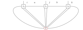
Semi-regularity yields one complementary virtual configuration for each region, so Theorem 38.9.20.19 identifies the two six-leg ranges with \(\mathcal K_{\widetilde A,R,C_L}\) and \(\mathcal K_{\widetilde A,S,C_R}\) without restricting their joint boundaries. By (260), their intersection is the range of the eight-leg map in (257), whose coordinate expansion is \(\zeta (X)\) in (262).
Let \(A\) be regular \(G\)-injective on a native torus with both periods at least three, with the same tensor repeated at every site. For each native plaquette \(R_v\), let \(P_v\geq 0\) have kernel equal to the image of the regional PEPS map, and put \(H=\sum _v(P_v\otimes \mathbf1_{R_v^c})\). In the coefficient form of [ 272 , Theorem 5.7 ] for this finite regular-torus setting, every vector \(\psi \in \ker H\), including zero, admits coefficients \(\mu _{g,h}\in \mathbb C\) such that
The parent kernel equals the span of the commuting closures. Since the indexing set of commuting pairs is finite, membership in this span gives (263).
Under the hypotheses of 38.9.20.22, suppose \(A\) is \(G\)-isometric. Let \(R\) have connected occupied nearest-neighbour graph and simply connected closed-cell realization, and let \(b\) count its crossing bonds. For \(\psi \in \ker H\setminus \{ 0\} \), let \(M_\psi (\sigma ,\tau )=\psi (\sigma \cup \tau )\) be its physical coefficient matrix across \(R\mid R^c\). There is one density matrix \(\rho _R\), independent of \(\psi \), such that \(\operatorname {tr}(M_\psi M_\psi ^\dagger ){\gt}0\) and
In this parent-ground-state form of [ 272 , Theorem 6.9 ] , the Rényi equality holds for every finite real \(\alpha \geq 0\).
Inserting (263) into \(M_\psi \) expresses it as a commuting-closure cut matrix. Restricting an arbitrary global configuration to \(R\) and \(R^c\) and reassembling it recovers that configuration, so \(M_\psi =0\) would imply \(\psi =0\). The common-density theorem for nonzero commuting-closure superpositions therefore applies.
Under the hypotheses of 38.9.20.23, let \(\psi ,\phi \in \ker H\setminus \{ 0\} \). Write \(\widehat M_\psi \) and \(\widehat M_\phi \) for their normalized physical coefficient matrices. Every operator \(O\) on \(R\) has equal normalized expectation, and some physical unitary \(U\) on \(R^c\) satisfies
In particular, the complement of the nonwrapping rectangle of sites with both coordinates nonzero is \(\{ (x,y):x=0\lor y=0\} \). As in [ 272 , Theorem 6.7 and Corollary 6.8 ] , a unitary on these two width-one stripes relates any two normalized nonzero parent ground states.
Expanding both ground vectors by (263) produces nonzero cuts by restriction and reassembly, to which the local-equivalence and stripe-unitary theorems apply.
Under the hypotheses of 38.9.20.22, let \(R\) have connected occupied graph and simply connected closed-cell realization. Let \(b\) count its crossing bonds and let \(\psi \in \ker H\setminus \{ 0\} \). Its normalized reduced density \(\rho _R=M_\psi M_\psi ^\dagger /\operatorname {tr}(M_\psi M_\psi ^\dagger )\) has positive denominator, is positive semidefinite with trace one, and satisfies
As in [ 272 , Corollary 6.10 ] for this regular native-torus scope, only \(G\)-injectivity is required.
Substituting (263) into the physical coefficient matrix expresses \(\psi \) as a nonzero closure superposition, to which the rank and zero-order entropy theorem applies.
38.9.21 Microscopic parent constraints and native seam boundaries
The parent-Hamiltonian argument in [ 272 ] uses the regional intersection and closure statements of Theorems 5.4 and 5.5. The auxiliary results below pass directly from microscopic plaquette constraints to boundary tensors on the original lattice.
Let \(\Gamma =(V,E)\) be a finite simple graph with ordered vertices. An edge \(e\) has tail \(t(e){\lt}h(e)\) and alphabet \(X_e=\{ 0,\ldots ,D_e-1\} \). Each site has its own tensor \(A_v\), with common physical codomain \(\mathbb C^d\) until the final theorem. For \(R\subseteq V\), define \(C_R=\{ e:\{ t(e),h(e)\} \not\subseteq R\} \). Replacing an incident edge by its unique endpoint at \(v\) identifies the original tensor coordinates with the independent endpoint coordinates. Thus contracting identity bonds gives exactly the original PEPS vector, and a diagonal endpoint assignment restricts to its original crossing labels. Write \(\mathcal S_{A,C}\) for the range of the cut contraction against one arbitrary joint boundary on the two incidences of each \(e\in C\).
Suppose \(D_e{\gt}0\) for every bond and that the finite family of regions \((R_i)_i\) covers \(V\). Let \(H_i\geq 0\) have kernel equal to the genuine open-region range on \(R_i\), and let \(H=\sum _i H_i\otimes I_{V\setminus R_i}\). Every \(\psi \in \ker H\) belongs to \(\bigcap _i\mathcal S_{A,C_{R_i}}\). Neither injectivity nor a common bond dimension is required.
Positivity places every regional slice in the corresponding open-region range, with a virtual boundary chosen jointly with the omitted physical coordinates. Closing both endpoints of each additional cut bond by an identity matrix makes the endpoint sum equal to the original graph sum; its exterior factor is \(\prod _{e\cap R_i=\varnothing }D_e\), which is nonzero and can be divided out. The resulting vector lies in the lifted regional range. Coverage forces every physical site slice into its tensor image. Independent local linear retractions then absorb the omitted physical factors into the same joint virtual boundary.
Let \(G\) be finite. Give each bond a matching semi-regular representation \(U_e\), and suppose each \(A_v\) is \(G\)-injective for its incident action. Suppose also that the covering region family is nonempty and covers every edge internally. Every physical parent vector admits canonical coordinates \(\xi \) recovered by \(\psi =(\bigotimes _v A_v)\xi \), with
Here \(b_p\) is the product of the matrices \(U_e(p_e)\) and \(c_p\) is the product trace-dual coefficient. One family of local inverses yields \(\xi \) and all its regional cut conditions simultaneously.
Semi-regularity gives a nonzero invariant vector on each bond, so every bond alphabet is nonempty, and the genuine local inverses apply to the boundaries obtained in Theorem 38.9.21.2. Every uncut bond has representation-matrix support. Edge coverage and the product-range characterization give one coherent bond expansion. The trace-dual identities extract its coefficients. A nonzero extracted coefficient of a regional cut must have one vertex-label realization on all its internal bonds. Applying the original invariant tensors recovers \(\psi \).
Let \(V=\mathbb Z_w\times \mathbb Z_h\) with \(w,h\geq 3\). The cut \(C_{c,r}\) consists exactly of the horizontal bonds from \((x,y)\) to \((x+1,y)\) with \(x+1=c\), and the vertical bonds from \((x,y)\) to \((x,y+1)\) with \(y+1=r\).
On this torus, let every \(U_e\) be semi-regular and every \(A_v\) be independently \(G\)-injective. Let \(H\) be any positive microscopic plaquette parent with the exact open-region kernels. Then \(\ker H\subseteq \mathcal S_{A,C_{c,r}}\) for every \(c,r\). The boundary correlates all exposed incidences, and the physical vector retains every original site.
The plaquettes cover all vertices and edges. For each nonzero coefficient in (270), regional vertex labels telescope around every plaquette, giving identity holonomy. Translating the tree gauge to the chosen origin \((c,r)\) sends all labels outside \(C_{c,r}\) to the identity. Applying the product of the local averages therefore turns each supported bond product into a cut contraction. The coherent sum lies in the same cut range. Finally the original site maps recover the physical vector.
Allow arbitrary finite physical alphabets \(Y_v\). Embed their tagged disjoint union in a common alphabet and let \(E_v:\mathbb C^{Y_v}\to \mathbb C^{\sum _w|Y_w|}\) be coordinate zero extension, with coordinate restriction \(R_vE_v=I\). Form the ordinary graph tensors \(B_v=E_vA_v\) and their positive plaquette parent \(H_B\). Every vector \(\Psi \) in the full ambient kernel has a unique original physical representative \(\psi \) satisfying
No restriction to the site images is imposed on \(\Psi \) beforehand.
Zero extension is injective and preserves \(G\)-injectivity. Each cut contraction commutes with the product of the physical extensions and restrictions. Vertex-covering parent constraints yield a cut representation of every ambient kernel vector; hence it lies in the product extension range. The product left inverse gives recovery and uniqueness. Applying Theorem 38.9.21.5 to \(B\) and restricting its boundary tensors to the original independent physical spaces yields the seam representations for \(\psi \).
One joint boundary on the original seam.
Fix \(C=C_{c,r}\) on the native torus with periods \(w,h\geq 3\). For each edge, let \(t(e){\lt}h(e)\) be its ordered graph orientation and \(X_e=\{ 0,\ldots ,D_e-1\} \). Write \(\alpha ^-=(\alpha ^-_e)_{e\in C}\) and \(\alpha ^+=(\alpha ^+_e)_{e\in C}\), each in \(\prod _{e\in C}X_e\). These are independent tuples at the tail and head incidences, respectively; they are not identified across a cut bond. For \(z\in \prod _{e\notin C}X_e\), let \(\eta _v(\alpha ^-,\alpha ^+,z)\) put \(\alpha ^-_e\) at \(t(e)\) and \(\alpha ^+_e\) at \(h(e)\) when \(e\in C\), and put the same \(z_e\) at both incidences when \(e\notin C\). Define
The box \(\mathcal K_{A,C}\) contains every microscopic site and exactly the uncut identity contractions. Its one physical leg denotes the entire tuple \(\sigma =(\sigma _v)_{v\in V}\in \prod _vY_v\).
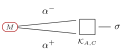
For the independently \(G\)-injective tensors and matching semi-regular bond representations of Theorem 38.9.21.5, every vector in the positive microscopic plaquette-parent kernel equals \(\mathcal C_{A,C}(M)\) for some such joint \(M\), at every choice of \(c,r\).
Padding leaves the joint boundary unchanged.
Put \(d=\sum _v|Y_v|\) and choose the tagged coordinate inclusion \(\iota _v:Y_v\hookrightarrow \{ 0,\ldots ,d-1\} \). Zero extension and restriction have coefficients \((E_v)_{j,i}=\delta _{j,\iota _v(i)}\) and \((R_v)_{i,j}=\delta _{\iota _v(i),j}\). Write \(E=\bigotimes _vE_v\), \(R=\bigotimes _vR_v\) and \(B_v=E_vA_v\). The physical tuples below are \(i=(i_v)\in \prod _vY_v\) and \(j=(j_v)\in \{ 0,\ldots ,d-1\} ^{V}\). For every joint \(M\), padding commutes with (273).
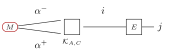 \(=\)
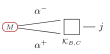
In particular, \(R\mathcal C_{B,C}(M)=\mathcal C_{A,C}(M)\) with exactly the same boundary coefficients.
Recovery on the full ambient parent kernel.
The identity \(R_vE_v=I\) implies \(RE\psi =\psi \) for every original physical vector \(\psi \); thus \(E\) is injective.
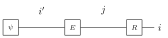 \(=\)

Conversely, let \(\Psi \in \ker H_B\) for the positive microscopic plaquette parent in Theorem 38.9.21.6. The parent constraints imply \(ER\Psi =\Psi \) without an assumed local-image condition.
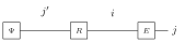 \(=\)

Thus the unique original representative is \(\psi =R\Psi \), and every native seam boundary for \(\Psi \) restricts to one for \(\psi \). The map \(ER\) is the coordinate projection onto \(\operatorname {ran}E\); padding is not assumed surjective onto the ambient physical space.
38.9.22 Nonuniform native parent classification
Let \(\Lambda =\mathbb Z_w\times \mathbb Z_h\) with \(w,h\geq 3\), and let \(E\) be the ordered edges of its native torus graph. Each edge \(e\) has its own finite virtual alphabet \(D_e\) and representation \(U_e\) of a finite group \(G\). Each vertex \(v\) has its own physical alphabet \(Y_v\) and tensor \(A_v\). The conclusions below give the native-simple-torus form of [ 272 , Theorems 5.7 and 5.9 ] , with no requirement that the representations, dimensions, or tensors be uniform.
Let \(\mathcal N_A(B)\) denote the contraction with bond matrices \(B_e\), acting from the tail index to the head index. Write \(p^{g,k}_e\) for the native closure labels: the ordered horizontal wrapping edges carry \(k^{-1}\), the ordered vertical wrapping edges carry \(g\), and other edges carry \(1\). Define
The local virtual alphabet is the product of the incident \(D_e\). The canonical tensor at \(v\) is the averaging projector \(P_v\) for its incident representation; write \(A^0_v=P_v\) and \(P=\bigotimes _vP_v\).
Given independent physical maps \(F_v\), finite physical alphabets give \(\zeta _{FA}(g,k)=(\bigotimes _vF_v)\zeta _A(g,k)\) and \(\mathcal Z_{FA}=(\bigotimes _vF_v)\mathcal Z_A\). If the original site maps \(T_v\) are invariant, \(T_vP_v=T_v\), so \(\mathcal Z_A=(\bigotimes _vT_v)\mathcal Z_{A^0}\).
Interchanging the finite physical sums with the bond contraction and using \(T_vP_v=T_v\) recovers every original site coefficient.
For the next regional-parent statements, take the physical alphabets to be a common finite alphabet. Independent physical alphabets are treated by Theorem 38.9.22.10.
On any finite ordered graph, suppose \(B_e=1\) for every edge internal to a region \(R\). Every exterior physical slice of \(\mathcal N_A(B)\) lies in the open-region range \(\mathcal S_{A,R}\). In addition, invariant tensors satisfy
Neither assertion assumes semi-regularity or injectivity.
Splitting the endpoint indices into internal and noninternal edges, the internal identities equate their two endpoints and leave the open-region contraction, while summing the noninternal indices yields its boundary coefficient. For (275), averaging the site representations, changing the vertex labels in the finite gauge sum, and using \(T_vP_v=T_v\) gives the invariance.
If each \(A_v\) is invariant, every commuting closure lies in every microscopic plaquette parent space. For the plaquette based at \(v=(x,y)\), the seams at \(x+2\) and \(y+2\) meet no internal edge. Consequently \(\mathcal Z_A\subseteq \bigcap _v\mathcal S_{A,R_v}^{\mathrm{ext}}\), where \(R_v=\{ x,x+1\} \times \{ y,y+1\} \) and the superscript denotes all exterior physical slices.
The native rightward bond label is \(k\) on its seam and the upward bond label is \(g^{-1}\) on its seam, so their square holonomy is the identity when \(gk=kg\). The translated tree gauge moves both seams to \(x+2,y+2\); since neither coordinate equals either coordinate of the plaquette, all internal bond matrices become identities, and local regional support followed by linear combinations gives the inclusion.
Suppose every \(U_e\) is semi-regular and every \(A_v\) is \(G\)-injective. Then \(\bigcap _v\mathcal S_{A,R_v}^{\mathrm{ext}}\subseteq \mathcal Z_A\). More precisely, for every flat bond assignment \(p\) there is a commuting pair \((g,k)\) such that \(PB(p)=\zeta _{A^0}(g,k)\), where \(B(p)\) is the product of the represented bond entries.
For a parent vector \(\psi \), the common local inverses give \(\xi \) with \(P\xi =\xi \), \((\bigotimes _vT_v)\xi =\psi \), and \(\xi =\sum _pc_pB(p)\). Regional trace-dual support makes every \(p\) with \(c_p\ne 0\) a vertex coboundary on each plaquette, hence flat. Its tree gauge leaves precisely two commuting seam holonomies. Gauge invariance of the site average gives
For closure evaluation and independence, allow independent physical alphabets \(Y_v\) again. These assertions concern the dependent contractions and do not require a new parent definition.
Local invariance gives \(\zeta _A(xgx^{-1},xkx^{-1})=\zeta _A(g,k)\). If all \(U_e\) are semi-regular, the native product trace-dual functional \(E_{a,b}\) satisfies
These equalities do not require \(g\) and \(k\) to commute.
The trace-dual pairings convert the local average into a sum over vertex labels \(q\), supported on \(p^{a,b}_e=q_{\mathrm{head}(e)}p^{g,k}_eq_{\mathrm{tail}(e)}^{-1}\). Off the seams these equations force neighboring \(q_v\) to coincide; nonseam connectivity therefore gives \(q_v=x\) everywhere. The two wrapping edges give \(a=xgx^{-1}\) and \(b=xkx^{-1}\), proving (277). On the diagonal the allowed \(x\) form the common centralizer, which contains identity. Constant gauge transformations and physical recovery prove the conjugacy invariance for the original tensors.
For a simultaneous-conjugacy class \(C=[(g,k)]\), put \(\zeta _A(C)=\zeta _A(g,k)\). This is well-defined. The set of closures indexed by commuting pairs equals the set indexed by commuting pair-conjugacy classes.
Suppose every \(U_e\) is semi-regular, all \(Y_v\) are finite, and every \(A_v\) is \(G\)-injective. The closure vectors belonging to distinct pair-conjugacy classes are linearly independent. In particular, \(\dim \mathcal Z_A=K\), where \(K\) is the number of simultaneous-conjugacy classes of commuting pairs.
Each functional in (277) vanishes on the other classes and is nonzero on its own class, so the canonical class vectors are independent. The product of genuine local \(G\)-injective inverses maps each original closure to its canonical closure and preserves independence; restricting to commuting classes and counting this independent spanning family gives \(\dim \mathcal Z_A=K\).
Take the physical alphabets to be a common finite alphabet. For each plaquette choose any positive interaction \(H_v\) with kernel exactly its open-region range, and extend it by identity to the other sites. Under the preceding semi-regularity and \(G\)-injectivity assumptions, the genuine microscopic Hamiltonian \(H=\sum _vH_v^{\mathrm{ext}}\) satisfies \(\ker H=\mathcal Z_A\) and \(\dim \ker H=K\). This includes the canonical orthogonal-complement interactions of [ 272 , Theorems 5.7 and 5.9 ] .
Positivity identifies \(\ker H\) with the intersection of the local parent spaces. The two inclusions identify that intersection with \(\mathcal Z_A\), whose dimension was calculated above.
Now allow arbitrary finite \(Y_v\). Let \(E_v\) be the zero extension of \(Y_v\) into the common tagged alphabet \(\coprod _vY_v\), and let \(R_v\) restrict to its tagged coordinates. Put \(E=\bigotimes _vE_v\), \(R=\bigotimes _vR_v\), and \(\widetilde A_v=E_vA_v\). Every positive microscopic parent \(\widetilde H\) of these padded tensors has full ambient kernel
Every ambient kernel vector \(\Psi \) therefore has a unique original representative \(\psi \in \mathcal Z_A\) with \(E\psi =\Psi \), and \(\dim \ker \widetilde H=K\). No support restriction is imposed on \(\Psi \).
Zero extension preserves \(G\)-injectivity and commutes with every native closure, so \(\mathcal Z_{\widetilde A}=E\mathcal Z_A\), and the native kernel theorem applied to the padded graph tensor gives \(\ker \widetilde H=E\mathcal Z_A\). Since \(RE=1\) on the full original physical space, \(E\) is injective, while the kernel equality makes it surjective onto the full ambient kernel, where \(ER=1\); these inverse maps preserve the dimension.