39 Angular information, regularized patch filters, and safe-box models
This chapter develops the nested-cylinder orthogonalization, annular angular-information bounds, and regularized patch-filter minimizers of [ 287 , Sections 3 and 4 ] , together with the finite-domain lattice models and safe-box exponent bootstrap shared with [ 286 ] .
39.1 Orthogonalization of nested cylinders
Let \(V\) be a finite set of sites, let \(\mathcal H_v\) be finite-dimensional coordinate Hilbert spaces, and write \(\mathcal H_R=\bigotimes _{v\in R}\mathcal H_v\). The empty tensor product is \(\mathbb {C}\). We use the natural regrouping \(\mathcal H_V=\mathcal H_R\otimes \mathcal H_{V\setminus R}\). The following construction is the orthogonalization step in the proof of the adaptive patch constraint in the September 24, 2026 polynomial-PEPS manuscript. It applies to arbitrary nested regions and inside subspaces.
For \(S\subseteq \mathcal H_R\), its cylinder is \(\mathcal C_R(S)=S\otimes \mathcal H_{V\setminus R}\). Equivalently, a vector belongs to \(\mathcal C_R(S)\) precisely when every slice at a fixed complementary coordinate belongs to \(S\). The inside rank of the specified pair \((R,S)\) is \(\dim S\); this is distinct from the dimension of the cylinder. In particular, \(\mathcal C_R(0)=0\).
Let \(A\) act on \(\mathcal H_R\), and let \(P_S\) be the orthogonal projector onto \(S\subseteq \mathcal H_R\). Then
Each complementary slice of \((A\otimes I)x\) is \(A\) applied to the corresponding slice of \(x\). Conversely, choose a preimage under \(A\) for each complementary slice and join these slices into one vector. This proves (1). The identity extension of \(P_S\) is self-adjoint and idempotent, with the required range, proving (2).
For a finite family of subspaces \(S_i\subseteq \mathcal H_R\), a linear operator \(A\) on \(\mathcal H_R\), and \(R\subseteq U\subseteq V\),
Decompose each complementary slice to prove the sum identity for two subspaces, then use finite induction. For images, use \(AS=\operatorname {ran}(AP_S)\) and (1). For containing regions, extend \(P_S\) first to \(U\) and then to \(V\); the composite extension is \(P_S\otimes I_{V\setminus R}\).
Let \(R_0\subseteq \cdots \subseteq R_{n-1}\) and \(S_j\subseteq \mathcal H_{R_j}\). Set \(\mathcal C_j=\mathcal C_{R_j}(S_j)\). For \(0\leq j{\lt}n\), define
When \(n{\gt}0\), we have \(W_0=0\) and \(\widetilde S_0=S_0\).
For \(0\leq j{\lt}n\), write \(\mathcal E_{j-1}=\sum _{i{\lt}j}\mathcal C_i\). Then
If \(S_j\subseteq W_j\), then \(\widetilde S_j=0\).
Extend the defining sum for \(W_j\) from \(R_j\) to \(V\). Equations (3) and (5) identify its cylinder with \(\sum _{i{\lt}j}\mathcal C_i\). By (4), the cylinder of \((I-P_{W_j})S_j\) is the image of \(\mathcal C_j\) under \((I-P_{W_j})\otimes I_{V\setminus R_j}\). Equation (2) identifies this operator with \(I_V-P_{\mathcal E_{j-1}}\). Finally, if \(s\in S_j\subseteq W_j\), then \(P_{W_j}s=s\), so \((I-P_{W_j})s=0\).
The spaces \(\widetilde{\mathcal C}_j\) are pairwise orthogonal. For every integer \(k\geq 0\), with summation indices restricted to \(0\leq j{\lt}n\),
Each inside rank satisfies \(\dim \widetilde S_j\leq \dim S_j\), and hence \(\sum _j\dim \widetilde S_j\leq \sum _j\dim S_j\).
By (10), every vector in the new cylinder is obtained by subtracting its projection onto the earlier span. For \(x\in \mathcal C_j\), decompose \(x=P_{\mathcal E_{j-1}}x+(I-P_{\mathcal E_{j-1}})x\). This gives
The new range is orthogonal to the earlier span because \(P_{\mathcal E_{j-1}}(I-P_{\mathcal E_{j-1}})=0\). Induction on the index gives equality of the original and new prefix spans. Every earlier new cylinder lies in the earlier original span, proving pairwise orthogonality. Finally, apply the image-dimension inequality to (7) inside \(\mathcal H_{R_j}\) and sum over \(j\).
Put \(\mathcal E=\sum _{j{\lt}n}\mathcal C_j\). Its orthogonal projector is
Distinct summands have product zero. For any finite family of regions, even without nesting, if every \(R_j\subseteq U\), the projector onto \(\sum _j\mathcal C_j\) is supported on \(U\): there is an orthogonal projector \(B\) on \(\mathcal H_U\) whose identity extension is that projector.
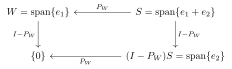
In \(\mathbb {C}^2\), let \(W=\operatorname{span}\{ e_1\} \) and \(S=\operatorname{span}\{ e_1+e_2\} \). Then \((I-P_W)S=\operatorname{span}\{ e_2\} \), whereas \(S\cap W^\perp =0\). The compression \((I-P_W)P_S(I-P_W)=\tfrac 12 P_{\operatorname{span}\{ e_2\} }\) is not idempotent, so it is not the projector onto the projected image. The diagram records the restrictions of the two orthogonal projections. The generator \(e_1+e_2\) maps to \(e_1\) and \(e_2\), respectively.
39.2 A uniform width bound for angular reset scales
Fix real constants \(C_3,C_4,K\) and a positive constant \(c\). The angular information argument bounds the reset width at scale \(s\) by
All powers in this section are real powers. The estimates below are used only for \(L\ge 2\) and \(s\ge 1\), where their bases are positive. They formalize the uniform scale argument following equation info-reset-scale-cost in the September 24, 2026 polynomial-PEPS manuscript. The source has nonnegative coefficients and exponent; the analytic bounds allow arbitrary fixed real values.
Let \(k=\lceil K\rceil _+=\max \{ 0,\lceil K\rceil \} \), and put
the explicit threshold beyond which \(\max \{ C_3,0\} (\log x)^K\le \frac{c}{2e}x\). The polylogarithmic scale and, for a slope \(D\), the size threshold are
Then \(S(K,C_3,c)\ge 1\) and \(L_{\rm w}(K,C_3,c,D)\ge 2\). For \(0{\lt}D\le D'\) one has \(L_{\rm w}(K,C_3,c,D')\le L_{\rm w}(K,C_3,c,D)\).
Let \(K,C_3\in \mathbb R\) and \(c{\gt}0\). For every \(s\ge S(K,C_3,c)\), the bound (15) holds.
Put \(x=es\), so that \(x\ge L_*\) and \(\log x=1+\log s\ge 1\). The explicit comparison of a real power of the logarithm with a larger power gives \(\max \{ C_3,0\} (1+\log s)^K\le \frac{c}{2e}\, es=\frac c2s\), and \(C_3\le \max \{ C_3,0\} \).
There is a real \(S\ge 1\) such that, for every \(s\ge S\),
Take \(S=S(K,C_3,c)\ge 1\) in Theorem 39.2.2.
Fix \(D{\gt}0\) with \(D\ge 4C_4/c\). For every real \(L\ge L_{\rm w}(K,C_3,c,D)\) one has \(e^{\max (K,1)}\le D\log L\), and for every real \(s\ge D\log L\),
Set \(T=\max \{ S(K,C_3,c),e^{\max (K,1)}\} \). Since \(L\ge e^{T/D}\) and \(L\ge 2\), \(D\log L\ge T\), so every \(s\ge D\log L\) satisfies \(s\ge S(K,C_3,c)\) and, by Theorem 39.2.2, its polylogarithmic term is at most \(cs/2\). The assumption \(D\ge 4C_4/c\) and \(\log L\ge 0\) give \(C_4\log L\le (c/4)D\log L\le cs/4\). Adding the two bounds proves the first inequality, and the second is strict because \(c{\gt}0\) and \(s\ge 1\).
Fix \(D{\gt}0\) with \(D\ge 4C_4/c\). There is a real \(L_0\ge 2\) such that, for every real \(L\ge L_0\), one has \(e^{\max (K,1)}\le D\log L\), and for every real \(s\ge D\log L\),
In particular one can choose \(D=\max \{ 1,4C_4/c\} \) before choosing \(L_0\). Once the coefficients and exponent are fixed, both choices are independent of \(L\) and \(s\).
Take \(L_0=L_{\rm w}(K,C_3,c,D)\ge 2\) in Theorem 39.2.4; for the second statement take \(D=\max \{ 1,4C_4/c\} \).
Fix \(D{\gt}0\) with \(D\ge 4C_4/c\). For every real \(L\ge L_{\rm w}(K,C_3,c,D)\), every real \(s\ge D\log L\) and every real \(w\le B(L,s)\), one has \(w{\lt}cs\).
Theorem 39.2.4 gives \(w\le B(L,s)\le \frac{3c}{4}s{\lt}cs\).
With the same fixed constants, any width function bounded above by \(B(L,s)\) is strictly smaller than \(cs\) throughout the stated range.
Take \(L_0=L_{\rm w}(K,C_3,c,D)\ge 2\) in Corollary 39.2.6.
39.3 Annular layers and ambient cell clearance
The plane carries the maximum metric. Let \(X,E\subseteq \mathbb R^2\), let \(\mathcal V\) be a finite set of marked points, and fix \(0{\lt}t\le n\). The construction below is the geometric part of Proposition 3.4 in the September 24, 2026 polynomial-PEPS manuscript.
For a real number \(n\) and an integer \(j\ge 0\), set \(s_j=n/2^j\). Then \(s_0=n\) and \(s_{j+1}=s_j/2\), equivalently \(2s_{j+1}=s_j\).
If \(n{\gt}0\), every \(s_j\) is positive. If \(n\ge 0\), every \(s_j\) is nonnegative, \(s_j\le s_i\le n\) for \(0\le i\le j\), and \(2s_j\le n\) for \(j{\gt}0\).
The denominator \(2^j\) is positive. For \(n\ge 0\), the identity \(s_{j+1}=s_j/2\) gives \(s_{j+1}\le s_j\); induction yields the asserted monotonicity and \(s_j\le s_0=n\). If \(j=k+1\), then \(2s_j=s_k\le n\).
For \(x\in \mathbb R^2\), put \(\delta (x)=\min (\{ n\} \cup \{ \operatorname {dist}_{\infty }(x,v):v\in \mathcal V\} )\). Thus \(\delta (x)=n\) for \(\mathcal V=\varnothing \); otherwise \(\delta (x)=\min \{ n,\operatorname {dist}_{\infty }(x,\mathcal V)\} \).
For any real \(r\), the inequality \(r\le \delta (x)\) holds exactly when \(r\le n\) and \(r\le \operatorname {dist}_{\infty }(x,v)\) for every \(v\in \mathcal V\). In particular, \(\delta (x)\le n\) and \(\delta (x)\le \operatorname {dist}_{\infty }(x,v)\) for every mark \(v\); if \(n\ge 0\), then \(\delta (x)\ge 0\). If \(r\le n\), then
A lower bound for the minimum of a nonempty finite set is exactly a lower bound for every element. The minimum is at most each element, and all elements are nonnegative when \(n\ge 0\). If \(r\le n\) and every marked-point distance were at least \(r\), the minimum would also be at least \(r\). Conversely, a marked-point distance below \(r\) bounds the minimum from above, proving (17).
There is an integer \(m\ge 0\) such that the scales \(s_j=n/2^j\) satisfy \(t\le s_m{\lt}2t\). For \(0\le j\le m\), one has \(s_j\ge t\). Fix one such stopping index \(m\) for the layer construction.
For an integer \(m\ge 0\) with \(2^m\le n/t{\lt}2^{m+1}\), dividing by the positive quantities \(t\) and \(2^m\) gives \(t\le s_m{\lt}2t\), and the decreasing property of \(s_j\) yields \(s_j\ge s_m\ge t\) for \(0\le j\le m\).
If \(m=0\), set \(B_0=X\). If \(m\ge 1\), define
Let \(A_j=\bigcup _{i\le j}B_i\) be the processed set. Put \(B_j=\varnothing \) for \(j{\gt}m\), so every \(B_j\) is a subset of \(X\). For \(m{\gt}0\), the first layer can equivalently be written as \(B_0=\{ x\in X:\operatorname {dist}_{\infty }(x,v)\ge n \text{ for every }v\in \mathcal V\} \).
For \(0{\lt}j{\lt}m\), a point belongs to \(B_j\) exactly when it belongs to \(X\), has distance at least \(s_j\) from every mark, and has distance less than \(2s_j\) from some mark. If \(m{\gt}0\), membership in \(B_m\) is equivalent to belonging to \(X\) and having distance less than \(2s_m\) from some mark. In particular, whenever \(j{\gt}0\) and \(x\in B_j\), there is \(v\in \mathcal V\) with \(\operatorname {dist}_{\infty }(x,v){\lt}2s_j\).
The inequalities \(s_j\le n\) and \(2s_j\le n\) for \(j{\gt}0\) allow both thresholds to be expressed through the marked-point distances using Theorem 39.3.4. The final layer has only the strict upper threshold; every positive-index layer retains this upper threshold, which yields the asserted mark.
One has \(A_0=B_0\), \(B_j\subseteq A_j\subseteq X\), and \(A_i\subseteq A_j\) whenever \(i\le j\). For every \(j\ge 0\), \(A_{j+1}=A_j\cup B_{j+1}\). For \(0\le j\le m\),
The union defining \(A_j\) gives the inclusions, monotonicity, and successor identity. If \(x\in B_i\) with \(i\le j\le m\), then either \(i=m\), which forces \(j=m\), or \(\delta (x)\ge s_i\ge s_j\). The reverse inclusion in (21) follows by induction on \(j\), where the base case \(j=0\) is the first or sole layer. At \(j+1\), a point with \(\delta (x)\ge s_j\) is already in \(A_j\) by induction. Otherwise \(\delta (x){\lt}s_j=2s_{j+1}\), and the assumed lower threshold, or the equality \(j+1=m\), places it in \(B_{j+1}\).
The angular separation condition for \(X\), \(E\), and a real constant \(a\) is the pairwise bound
for every \(x\in X\) and \(y\in E\). This condition is vacuous if either set is empty.
The layers are pairwise disjoint and \(A_m=X\). If \(a\ge 0\) and \(\operatorname {dist}_{\infty }(x,y)\ge a\max \{ t,\delta (x)\} \) for all \(x\in X\) and \(y\in E\), then for \(0\le j\le m\), every \(x\in A_j\) and \(y\in E\) satisfy \(\operatorname {dist}_{\infty }(x,y)\ge as_j/2\). For \(j{\lt}m\) the stronger bound \(as_j\) holds. If \(\mathcal V=\varnothing \), then \(B_0=X\) and all later layers are empty. Thus each \(x\in X\) belongs to a layer \(B_j\) with \(j\le m\), and \(A_j\cap B_{j+1}=\varnothing \) for every \(j\ge 0\).
The equality \(2s_{j+1}=s_j\) and the strict upper boundary in (20) give disjointness. Induction on \(j\) gives \(A_j=\{ x\in X:\delta (x)\ge s_j\} \) for \(j{\lt}m\), and \(A_m=X\). Before the last scale, \(\max \{ t,\delta (x)\} \ge s_j\). At the last scale it is at least \(t{\gt}s_m/2\). When the marked set is empty, \(\delta (x)=n\) and \(2s_j\le n\) for \(j{\gt}0\).
For an origin \(o\in \mathbb R^2\), side \(q{\gt}0\) and \(i\in \mathbb Z^2\), let \(Q_i=o+q(i+[0,1)^2)\). The owner of \(x\) has coordinates \(\lfloor (x_k-o_k)/q\rfloor \). For any set \(A\), write \(A^{+r}=\bigcup _{x\in A}\overline B_\infty (x,r)\). Select precisely the cells meeting \(A^{+r}\), and denote their union by \(U_{q,r}(A)\). Write \(\iota (x)\) for the owner and \(I_{q,r}(A)=\{ i\in \mathbb Z^2:Q_i\cap A^{+r}\ne \varnothing \} \) for the selected indices. The grid origin is fixed in this notation.
Every point \(x\) belongs to \(Q_{\iota (x)}\). If \(x\in Q_i\), then \(i=\iota (x)\); hence \(x\in Q_i\cap Q_j\) implies \(i=j\). For \(x,y\in Q_i\), one has \(\operatorname {dist}_{\infty }(x,y)\le q\).
For each coordinate, the floor inequality \(\lfloor (x_k-o_k)/q\rfloor \le (x_k-o_k)/q {\lt}\lfloor (x_k-o_k)/q\rfloor +1\) gives membership after multiplication by \(q{\gt}0\). Conversely, the defining inequalities for \(Q_i\) identify this floor with \(i_k\). Two coordinates in the same half-open interval of length \(q\) differ in absolute value by at most \(q\), so their maximum does also.
For \(j\in \mathbb Z^2\), an integer \(N\ge 0\), and a finite set \(F\subseteq \mathbb R^2\), define
One has \(|H_N(j)|=(2N+3)^2\) and \(|\mathcal C_N(F)|\le |F|(2N+3)^2\). If \(x\in Q_i\) and \(\operatorname {dist}_{\infty }(x,c)\le u\le Nq\), then \(i\in H_N(\iota (c))\).
Each coordinate interval defining \(H_N(j)\) contains \(2N+3\) integers. Multiplying the two counts proves the exact cardinality, and the cardinality of a finite union is at most the sum of the cardinalities. For the last assertion, with \(j=\iota (c)\) so that \(c\in Q_j\), the inequalities defining \(Q_i\) and \(Q_j\), together with \(|x_k-c_k|\le u\le Nq\), give \((j_k-N-1)q{\lt}i_kq{\lt}(j_k+N+1)q\) for each coordinate \(k\). Division by \(q{\gt}0\) gives the required non-strict integer bounds.
Suppose \(A\) is covered by the closed radius-\(R\) squares centered at a finite set \(F\). If \(R+r\le Nq\) for an integer \(N\ge 0\), then \(I_{q,r}(A)\subseteq \mathcal C_N(F)\). In particular, \(I_{q,r}(A)\) is finite and \(|I_{q,r}(A)|\le |F|(2N+3)^2\). If instead the covering radius is \(Rs\), where \(d,s{\gt}0\), set \(q=ds\) and \(N=\lceil (R+r)/d\rceil _+\), where \(\lceil u\rceil _+\) is the least nonnegative integer at least \(u\). Then \(I_{ds,rs}(A)\subseteq \mathcal C_N(F)\) for this grid, and
For a selected index \(i\), there exist \(y\in Q_i\), \(x\in A\) with \(\operatorname {dist}_{\infty }(y,x)\le r\), and a cover center \(c\in F\) with \(\operatorname {dist}_{\infty }(x,c)\le R\). The triangle inequality gives \(\operatorname {dist}_{\infty }(y,c)\le R+r\le Nq\). Theorem 39.3.14 places \(i\) in \(H_N(\iota (c))\subseteq \mathcal C_N(F)\) and bounds the cardinality upon retaining the indices in \(\mathcal C_N(F)\) whose cells meet the enlargement. In the scaled case, the ceiling inequality gives \(Rs+rs=(R+r)s\le Nd s=Nq\), proving (25).
For arbitrary sets \(A,B\), one has \((A\cup B)^{+r}=A^{+r}\cup B^{+r}\). If \(A\subseteq B\) and \(r\le u\), then \(A^{+r}\subseteq B^{+u}\). For every \(q{\gt}0\),
Also \(A\subseteq B\) implies \(U_{q,r}(A)\subseteq U_{q,r}(B)\).
A center in \(A\cup B\) lies in one of the two sets, proving the union identity. Enlarging the center set and radius preserves the distance bound. A point of \(A^{+r}\) lies in its owner cell, which is selected. If \(x\in U_{q,r}(A)\), its cell contains a point \(y\) at distance at most \(r\) from some center \(z\in A\), and the cell diameter bound gives \(\operatorname {dist}_{\infty }(x,z)\le q+r\), proving (26). Any point showing that a cell meets \(A^{+r}\) also shows that it meets \(B^{+r}\) when \(A\subseteq B\).
Every cell selected from \(A\cup B\) but not from \(A\) is selected from \(B\). Suppose \(d,s{\gt}0\) and a finite set \(F\) of centers gives a closed radius-\(Rs\) square cover of \(B\). Then \(I_{ds,rs}(A\cup B)\setminus I_{ds,rs}(A)\) is finite and has cardinality at most \(|F|(2\lceil (R+r)/d\rceil _++3)^2\), with no cardinality assumption on the cells selected from \(A\).
A point of \(A\cup B\) within distance \(rs\) of the cell must lie in \(B\) if the cell is not selected from \(A\). By Theorem 39.3.15, the cells selected from \(B\) satisfy the stated finite bound, and retaining those not selected from \(A\) isolates the newly selected cells without increasing the cardinality.
Suppose \(\operatorname {diam}_{\infty }(X)\le A_0n\) and \(|\mathcal V|\le m_0\). Put \(R=\max \{ A_0,2\} \). Each \(B_j\) is covered by at most \(m_0+1\) closed squares of radius \(Rs_j\). It is therefore covered by at most \((m_0+1)(2\lceil R\rceil _++3)^2\) ambient cells of side \(s_j\). For \(d{\gt}0\), the cells of side \(ds_j\) meeting \(B_j^{+rs_j}\) form a finite set with cardinal at most
For \(1\le j\le m\), the same bound holds for the cells meeting \(A_j^{+rs_j}\) that do not meet \(A_{j-1}^{+rs_j}\). The bound is independent of \(j,n,o\), the marked points and the shapes of the sets.
For the first or sole layer, any \(x_0\in X\) (when \(X\) is nonempty) satisfies \(X\subseteq \overline B_\infty (x_0,A_0n)\) by the diameter bound, while an empty \(X\) is covered by the empty family. In a later layer, \(\delta (x){\lt}2s_j\le n\) gives some \(v\in \mathcal V\) with \(\operatorname {dist}_{\infty }(x,v){\lt}2s_j\).
A cell meeting a radius-\((R+r)s_j\) square has index within \(N+1\) in each coordinate of the center’s owner, where \(N=\lceil (R+r)/d\rceil _+\). There are \((2N+3)^2\) such indices, so taking the union over the cover centers and retaining the cells that meet the enlargement proves (27). Finally, \(A_j=A_{j-1}\cup B_j\) and enlargement commutes with union, so any newly selected cell meets \(B_j^{+rs_j}\).
Suppose \(q{\gt}0\) and \(b\le \operatorname {dist}_{\infty }(u,v)\) for every \(u\in A\) and \(v\in E\). For \(x\in U_{q,r}(A)\) and \(y\in E^{+\rho }\),
Independently, if \(x\in A^{+r}\) and \(y\notin A^{+\rho }\), then \(\rho -r{\lt}\operatorname {dist}_{\infty }(x,y)\).
For \(z\in A\) and \(w\in E\) with \(\operatorname {dist}_{\infty }(x,z)\le r+q\) and \(\operatorname {dist}_{\infty }(y,w)\le \rho \), the triangle inequality gives \(b\le \operatorname {dist}_{\infty }(z,w) \le r+q+\operatorname {dist}_{\infty }(x,y)+\rho \), proving (28). For the second assertion, picking \(z\in A\) with \(\operatorname {dist}_{\infty }(x,z)\le r\) shows that \(\operatorname {dist}_{\infty }(x,y)\le \rho -r\) would imply \(\operatorname {dist}_{\infty }(y,z)\le \rho \), contradicting \(y\notin A^{+\rho }\).
Let \(d,s{\gt}0\) and assume \((a/2)s\le \operatorname {dist}_{\infty }(u,v)\) for every \(u\in A\) and \(v\in E\). For \(x\in U_{ds,3a's/2}(A)\) and \(y\in E^{+3a's/2}\), one has \(\operatorname {dist}_{\infty }(x,y)\ge (a/2-3a'-d)s\). If also \(0{\lt}a'{\lt}a/100\) and \(d{\lt}a'/4\), then \(a/2-3a'-d{\gt}0\).
Substituting \(b=as/2\), \(q=ds\), and \(r=\rho =3a's/2\) into (28) yields the distance bound, and for \(a{\gt}100a'\) and \(d{\lt}a'/4\) we have \(a/2-3a'-d{\gt}(50-3-1/4)a'{\gt}0\).
Assume \(\operatorname {dist}_{\infty }(x,y)\ge a\max \{ t,\delta (x)\} \) for every \(x\in X\) and \(y\in E\). Fix \(0\le j\le m\), \(0{\lt}a'{\lt}a/100\), \(0{\lt}d{\lt}a'/4\) and \(s=s_j{\gt}0\). Let \(U=U_{ds,3a's/2}(A_j)\), and let \(\Lambda \) be any physical domain. Set \(R_\Lambda =\Lambda \cap U\) and \(C_\Lambda =\Lambda \cap E^{+3a's/2}\). With \(A_{-1}=\varnothing \) at the initial step, the selected old group is contained in \(A_{j-1}^{+2a's}\), and \(E^{+3a's/2}\subseteq E^{+2a's}\). Every \(x\in U\) and \(y\in E^{+3a's/2}\) satisfy
Thus \(R_\Lambda \) and \(C_\Lambda \) are disjoint. Both cores \(\Lambda \cap A_j^{+a's}\) and \(\Lambda \cap E^{+a's}\) are contained in their corresponding regions. Every core point is at distance greater than \(a's/2\) from every point of the corresponding physical complement.
Two points of one cell are at distance at most \(ds\), so \(U_{ds,3a's/2}(A)\subseteq A^{+(3a'/2+d)s}\subseteq A^{+2a's}\). The triangle inequality subtracts the two enlargement radii and one cell side from the separation \(as/2\), proving (29). The choice of constants makes its coefficient positive. Every point of \(A_j^{+3a's/2}\) lies in its selected owner cell. If a point within distance \(a's\) of a core center were at distance at most \(a's/2\) from an excluded point, that excluded point would belong to the closed radius-\(3a's/2\) enlargement, a contradiction. Intersecting with \(\Lambda \) preserves every inclusion and pairwise bound.
For fixed real \(K,C_3,C_4\) and \(a'{\gt}0\), there exist \(D\ge 1\) and \(L_0\ge 2\) such that \(D\ge 4C_4/(a'/3)\) and, for every \(L\ge L_0\) and \(s\ge D\log L\), \(C_3(1+\log s)^K+C_4\log L{\lt}(a'/3)s\).
Applying Theorem 39.2.5 with \(c=a'/3\) yields \(D\) and \(L_0\).
Let \(s,r,b\in \mathbb R\), and let \(Q_i\) be the cells defined by the coordinate inequalities of Definition 39.3.11. Let \(U\) be the union of the cells meeting \(A^{+r}\), and suppose that \(Q_i\) is one of these selected cells. To establish the closed-cell separation required in [ 287 , Lemma 3.2 and Proposition 3.4 ] , if \(\operatorname {dist}_\infty (x,y)\ge b\) for every \(x\in U\) and \(y\in C\), then the same inequality holds for every \(x\in \overline{Q_i}\) and \(y\in C\).
For any \(y\in C\), every point of \(Q_i\) belongs to \(U\), so its distance from \(y\) is at least \(b\). Because the set \(\{ x:\operatorname {dist}_\infty (x,y)\ge b\} \) is closed, it contains \(\overline{Q_i}\).
For a grid of side \(s{\gt}0\), a point \(x\) belongs to \(U_{s,r}(A)\) if and only if its cell index \(\iota (x)\) belongs to \(I_{s,r}(A)\).
If \(x\) lies in a selected cell \(Q_i\), uniqueness of the cell index gives \(i=\iota (x)\). Conversely, \(x\in Q_{\iota (x)}\), so selection of this cell implies membership in the selected union.
For \(L\in \mathbb N\) and \(x,y\in \{ 0,\ldots ,L-1\} ^2\), their physical positions \(x+(1,1)\) and \(y+(1,1)\) identify the distances in the geometric construction with those in the information reset of [ 287 , Lemma 3.3 ] via
Subtracting the coordinates cancels the common translation, leaving the maximum of the two absolute coordinate differences as the integer sup distance viewed as a real number.
39.4 Angular information under the sublinear collar bound
Fix \(q\in \mathbb N\), \(c{\gt}0\), a template constant \(C_{\rm tpl}\), a collar threshold \(N\), an amplification constant \(C_a\) and an amplification threshold \(N_a\), and recall \(\beta _0{\lt}1\). Let \(u_0=u_0(C_{\rm tpl},66^2,1,N,C_a,N_a)\) be the coarse threshold of Definition 42.11.6 and \(u_1=U(2/c,\beta _0,1)\) the power threshold of Theorem 42.2.4, so that \(2u^{\beta _0}\le cu\) for \(u\ge u_1\). The lower tile scale is \(u_{\rm cell}=\max \{ u_0,u_1\} \). With the partition constants of Definition 42.2.7, the cell prefactor and exponent are
For all values of the parameters, the cell prefactor \(C_{\rm cell}\) and the cell exponent \(K_{\rm cell}\) are positive.
The partition constants are positive by Theorem 42.2.8, and \(\max \{ 1,2\log q,\max \{ C_a,0\} \} \ge 1\).
In the conditional form of [ 287 , Lemma 3.2 ] (with the explicit collar hypothesis discussed in [ 293 ] ), fix \(q,R\in \mathbb N\), \(J,\Delta \in \mathbb R\) and template constants \(D_0,C_{\rm tpl}\). Suppose that the sublinear collar bound at range \(R\) holds with constant \(C\) and threshold \(N\), and that the amplification bound at range \(R\) holds at \((\max \{ C,1\} ,1)\) with constant \(C_a\) and threshold \(N_a\). The source has only site and nearest-neighbour terms, which is range one; ranges \(R{\gt}1\) extend it. Fix \(c{\gt}0\), and let \(C_{\rm cell},K_{\rm cell}\) be the constants of Definition 39.4.1. Let \(s\ge 1\), let \(o\in \mathbb R^2\) be a grid origin, and set \(Q_i=o+si+[0,s)^2\) for \(i\in \mathbb Z^2\). Choose an index \(i_0\) and any set of indices \(A\) with \(i_0\notin A\). On any finite integer domain \(\Lambda \), let \(H\) be a Hamiltonian of range \(R\) with interaction bound \(J\), and let \(\Omega \) be a unit ground vector with full-system gap \(\Delta \). Put \(G=\Lambda \cap Q_{i_0}\) and \(B=\Lambda \cap \bigcup _{i\in A}Q_i\). If \(E\subseteq \Lambda \setminus (G\cup B)\) and \(\operatorname {dist}_\infty (x,y)\ge cs\) for every \(x\in \overline{Q_{i_0}}\) and \(y\in E\), then
The coarse information estimate with explicit constants, for unions of at most \(66^2\) boxes of diameter at most the scale, gives the tile bound \(C_2=\max \{ C_a,0\} \) at every scale \(u\ge u_0\) and separation \(u^{\beta _0}\). The partition with explicit constants at the exponent \(\beta _0\) and the lower bound \(u_{\rm cell}\) has all tile scales at least \(u_{\rm cell}\), so both \(u\ge u_0\) and \(2u^{\beta _0}\le cu\) hold at every tile scale. Giving the cells indexed by \(A\) colour zero and the other exterior cells colour one, and restricting the ordered partition to \(\Lambda \), retains its order and families without increasing its residual cardinality. The separation of tiles of one family from their predecessors and from the corresponding exterior cells gives the two coarse information bounds. For the first family, the additional separation from \(E\) follows from \(u^{\beta _0}{\lt}cs\) and the closed-cell hypothesis. If \(N_{\rm t}\) is the number of tiles and \(D\) the residual, the counting form of the two-family inequality gives
where \(M=\max \{ 1,2\log q,C_2\} \), which is the stated bound.
In the conditional form of [ 287 , Lemma 3.2 ] (with the explicit collar hypothesis discussed in [ 293 ] ), fix \(q,R\in \mathbb N\), \(J\in \mathbb R\), \(\Delta {\gt}0\), and template constants for which the sublinear collar bound at range \(R\) holds, and fix \(c{\gt}0\). The source has only site and nearest-neighbour terms, which is range one; ranges \(R{\gt}1\) extend it. There exist \(C_1{\gt}0\) and \(K\ge 0\) with the following property. Let \(s\ge 1\), let \(o\in \mathbb R^2\) be a grid origin, and set \(Q_i=o+si+[0,s)^2\) for \(i\in \mathbb Z^2\). Choose an index \(i_0\) and any set of indices \(A\) with \(i_0\notin A\). On any finite integer domain \(\Lambda \), let \(H\) be a Hamiltonian of range \(R\) with interaction bound \(J\), and let \(\Omega \) be a unit ground vector with full-system gap \(\Delta \). Put \(G=\Lambda \cap Q_{i_0}\) and \(B=\Lambda \cap \bigcup _{i\in A}Q_i\). If \(E\subseteq \Lambda \setminus (G\cup B)\) and \(\operatorname {dist}_\infty (x,y)\ge cs\) for every \(x\in \overline{Q_{i_0}}\) and \(y\in E\), then
The constants precede the scale, grid, finite domain, Hamiltonian and ground vector.
Fix \(q\in \mathbb N\), \(J\in \mathbb R\), \(\Delta \in \mathbb R\) and template constants \(D_0,C_{\rm tpl}\). Suppose that the range-one sublinear collar bound holds with constant \(C\) and threshold \(N\), and that the range-one amplification bound holds at \((\max \{ C,1\} ,1)\) with constant \(C_a\) and threshold \(N_a\). Fix \(c{\gt}0\). The conclusion of Theorem 39.4.3 holds with the same constants \(C_{\rm cell},K_{\rm cell}\) of Definition 39.4.1 for the original open square \(\Lambda _L=\{ 1,\ldots ,L\} ^2\), every Hamiltonian of the square-grid model with interaction bound \(J\), and every unit ground vector with full-system gap \(\Delta \). The regions \(G,B,E\) are the same physical cell, conditioning union and exterior region, and the separation hypothesis concerns the full closed ambient cell.
Relabeling the square sites by the integer rectangle \(\{ 0,\ldots ,L-1\} ^2\) and replacing the grid origin \(o\) by \(o-(1,1)\) sends the chosen half-open cell and its closure to the original cell and closure under translation by \((1,1)\), while preserving distances. The relabeling preserves the Hamiltonian, ground-state equation and full-system gap, and carries both cell samples and the conditioning union to the original physical regions. Theorem 39.4.3 then applies, and because relabeling preserves each of the four regional entropies in \(I_\Omega (G:E\mid B)\), the stated bound holds for the same vector \(\Omega \).
Fix \(q\in \mathbb N\), \(J\in \mathbb R\) and \(\Delta {\gt}0\), and assume the range-one sublinear collar bound for fixed template constants. Fix \(c{\gt}0\). The conclusion of Theorem 39.4.4 holds with uniform constants \(C_1{\gt}0\), \(K\ge 0\) for the original open square \(\Lambda _L=\{ 1,\ldots ,L\} ^2\), every Hamiltonian of the square-grid model, and every unit ground vector with full-system gap \(\Delta \). The regions \(G,B,E\) are the same physical cell, conditioning union and exterior region, and the separation hypothesis concerns the full closed ambient cell. No restriction on the cardinality of any region is imposed. The collar hypothesis remains explicit, as in [ 293 ] .
For the finite cell addition in the proof of [ 287 , Proposition 3.4 ] , fix a grid origin \(o\), a side length \(s{\gt}0\), an enlargement radius \(r\), and \(c{\gt}0\). Write \(Q_i=o+si+[0,s)^2\) for \(i\in \mathbb Z^2\). Let \(A_{\rm old}\subseteq A\) be ambient sets and let \(S\) be the finite set of cells selected by \(A\) but not by \(A_{\rm old}\). Write \(R_{\rm old},R\) for the physical samples of their selected unions, and \(G_i\) for the physical sample of cell \(i\). Let \(\Omega \) be a vector on the square lattice and let \(E\) be a physical region at distance at least \(cs\) from every point of the selected union for \(A\).
Suppose that, for every \(i\in S\) and every union \(B\) of physical samples of cells other than \(i\), the conditions \(E\subseteq (G_i\cup B)^c\) and \(\operatorname {dist}_\infty (\overline{Q_i},E)\ge cs\) imply \(I_\Omega (G_i:E\mid B)\le k\). If \(I_\Omega (R_{\rm old}:E)\le b_0\), then
No normalization or sign assumption on \(k\) is required.
The selected region is exactly \(R_{\rm old}\cup \bigcup _{i\in S}G_i\). The unique cell index of each physical site identifies every intermediate conditioning region with a union of whole cells. Positive clearance makes \(E\) disjoint from these regions, and continuity of distance extends the clearance to each closed cell. The assumed conditional bound therefore applies at every addition. The entropy chain identity bounds the total increase by \(\sum _{i\in S}k=|S|k\).
Fix a local dimension \(q\ge 1\), an interaction bound \(J\ge 0\), a gap \(\Delta {\gt}0\), and \(p{\gt}0\), and let \(C_p=C_p(J,\Delta ,p)\) and \(L_0=L_0(q,J,\Delta ,p)\) be the reset width and size threshold of Definition 45.20.8. Let \(L\ge L_0\) and let \(\Omega \) be a normalized ground vector of the square Hamiltonian with interaction bound \(J\) and full-system gap \(\Delta \). Choose ambient sets \(A,E\), a grid origin, and parameters \(a'\ge 0\), \(d{\gt}0\), and \(s{\gt}0\). Let \(R\) be the physical sample of all cells of side \(ds\) meeting \(A^{+3a's/2}\), and let \(C=\Lambda _L\cap E^{+3a's/2}\). Put \(R_0=\Lambda _L\cap A^{+a's}\) and \(C_0=\Lambda _L\cap E^{+a's}\). Suppose \(R\cap C=\varnothing \), \(b\ge 0\), \(I_\Omega (R:C)\le b\) and \(C_p(1+b+\log L)\le a's/2\). Then \(I_\Omega (R_0:C_0)\le L^{-p}\).
Each core lies in its corresponding larger region and has distance strictly greater than \(a's/2\) from the corresponding physical complement. The common translation of physical lattice coordinates preserves the sup distance. The information reset theorem with explicit constants applies to the original Hamiltonian and ground vector with these two buffers.
For the regions used in [ 287 , Proposition 3.4 ] , fix a local dimension \(q\ge 1\), an interaction bound \(J\ge 0\), a gap \(\Delta {\gt}0\), and \(p{\gt}0\). There are constants \(C_p{\gt}0\) and \(L_0\) with the following property. Let \(L\ge L_0\) and let \(\Omega \) be a normalized ground vector of the square Hamiltonian with full-system gap \(\Delta \). Choose ambient sets \(A,E\), a grid origin, and parameters \(a'\ge 0\), \(d{\gt}0\), and \(s{\gt}0\). Let \(R\) be the physical sample of all cells of side \(ds\) meeting \(A^{+3a's/2}\), and let \(C=\Lambda _L\cap E^{+3a's/2}\). Put \(R_0=\Lambda _L\cap A^{+a's}\) and \(C_0=\Lambda _L\cap E^{+a's}\). Suppose \(R\cap C=\varnothing \), \(b\ge 0\), and
Then \(I_\Omega (R_0:C_0)\le L^{-p}\).
Take \(C_p=C_p(J,\Delta ,p){\gt}0\) and \(L_0=L_0(q,J,\Delta ,p)\) in Theorem 39.4.8.
For real numbers \(C_p,a',d,C_1,N,K\), put
with \(L_{\rm w}\) the size threshold of Definition 39.2.1. Then \(D_{\rm cell}\ge 1\) and \(L_{\rm cell}\ge e\). The slope satisfies \(D_{\rm cell}\ge 4C_p/c_*\) for the available width \(c_*=a'/3\) of [ 287 , Proposition 3.4 ] .
Fix \(a',C_p,C_1,p{\gt}0\), \(0{\lt}d\le 1\), and real numbers \(N,K\ge 0\), and let \(D\ge D_{\rm cell}(C_p,a',d)\). For all real \(L,s\) with \(L\ge L_{\rm cell}(a',d,C_p,C_1,N,K)\) and \(s\ge D\log L\), one has \(ds\ge 1\) and
Since \(D\ge D_{\rm cell}\ge 1\), the threshold \(L_{\rm w}\) at the slope \(D\) is at most the one at \(D_{\rm cell}\), hence at most \(L\), and \(D\ge 4C_p/(a'/3)\). The explicit fitting estimate applies with coefficients \(C_3=C_p(2+NC_1)\) and \(C_4=C_p\) and width \(c=a'/3\). Since \(L\ge e\), \(\log L\ge 1\), so \(s\ge D\ge 1/d\) gives \(ds\ge 1\), while \(L^{-p}\le 1\) and \((1+\log (ds))^K\le (1+\log s)^K\). Since \((1+\log s)^K\ge 1\), the required width is at most \(C_3(1+\log s)^K+C_4\log L\), which is strictly less than \(a's/3\).
For the uniform choice of scales in [ 287 , Proposition 3.4 ] , fix \(a',C_p,C_1,p{\gt}0\), \(0{\lt}d\le 1\), and real numbers \(N,K\ge 0\). There are \(D\ge 1\) and \(L_0\ge e\) such that, for all real \(L,s\) with \(L\ge L_0\) and \(s\ge D\log L\), one has \(ds\ge 1\) and
Take \(D=D_{\rm cell}(C_p,a',d)\) and \(L_0=L_{\rm cell}(a',d,C_p,C_1,N,K)\) in Theorem 39.4.11.
Fix \(q\in \mathbb N\), \(J\in \mathbb R\), \(\Delta \in \mathbb R\) and template constants \(D_0,C_{\rm tpl}\). Suppose that the range-one sublinear collar bound holds with constant \(C\) and threshold \(N\), and that the range-one amplification bound holds at \((\max \{ C,1\} ,1)\) with constant \(C_a\) and threshold \(N_a\). Fix \(c{\gt}0\), and let \(C_{\rm cell},K_{\rm cell}\) be the constants of Definition 39.4.1 at this \(c\). Let \(s\ge 1\), let \(o\in \mathbb R^2\) be a grid origin, let \(r\in \mathbb R\), and let \(A_{\rm old}\subseteq A\) be ambient sets. Let \(S\) be a finite set of cell indices consisting exactly of the cells of side \(s\) meeting \(A^{+r}\) but not \(A_{\rm old}^{+r}\). On the original open square \(\Lambda _L=\{ 1,\ldots ,L\} ^2\), let \(H\) have interaction bound \(J\) and let \(\Omega \) be a unit ground vector with full-system gap \(\Delta \). Write \(R_{\rm old}\) and \(R\) for the physical samples of the two selected unions. Let \(E\subseteq \Lambda _L\) have distance at least \(cs\) from every point of the ambient selected union for \(A\). If \(I_\Omega (R_{\rm old}:E)\le b_0\), then
The square-grid cell estimate with explicit constants applies to every new cell conditioned on any union of the other whole cells, with the same vector \(\Omega \) and exterior \(E\). The selected-cell summation theorem therefore gives \(I_\Omega (R:E)\le b_0+\sum _{i\in S}C_{\rm cell}(1+\log s)^{K_{\rm cell}}\).
In the conditional step of [ 287 , Proposition 3.4 ] (with the collar hypothesis remaining explicit, as recorded in [ 293 ] ), fix \(q\in \mathbb N\), \(J\in \mathbb R\), \(\Delta {\gt}0\) and fixed template constants for which the range-one sublinear collar bound holds, and fix \(c{\gt}0\). There exist \(C_1{\gt}0\) and \(K\ge 0\) with the following property. Let \(s\ge 1\), let \(o\in \mathbb R^2\) be a grid origin, let \(r\in \mathbb R\), and let \(A_{\rm old}\subseteq A\) be ambient sets. Suppose that the set \(S\) of cells selected by \(A\) but not by \(A_{\rm old}\) is finite. On the original open square \(\Lambda _L=\{ 1,\ldots ,L\} ^2\), let \(H\) have interaction bound \(J\) and let \(\Omega \) be a unit ground vector with full-system gap \(\Delta \). Write \(R_{\rm old}\) and \(R\) for the physical samples of the two selected unions. Let \(E\subseteq \Lambda _L\) have distance at least \(cs\) from every point of the ambient selected union for \(A\). If \(I_\Omega (R_{\rm old}:E)\le b_0\), then
The constants precede the grid, ambient sets, square size, Hamiltonian, ground vector and exterior region.
The collar bound holds with some constant \(C\) and threshold \(N\), and the amplification bound at \((\max \{ C,1\} ,1)\) holds with some constant \(C_a\) and threshold \(N_a\). Take \(C_1=C_{\rm cell}{\gt}0\) and \(K=K_{\rm cell}{\gt}0\) in Theorem 39.4.13.
Let \(\Omega \) be a unit vector on a finite physical square \(\Lambda \), and let \(X,E\subseteq \Lambda \). Identify the sites with their integer positions in the plane, and take all enlargements in the ambient \(\ell _\infty \) metric before intersecting with \(\Lambda \). Let \(n{\gt}0\), \(a\geq 0\), \(\varepsilon \geq 0\), \(0{\lt}a'{\lt}a/100\), and \(0{\lt}d{\lt}a'/4\). Suppose that \(X\) has diameter at most \(A_0n\), that the marked set has at most \(m_0\) points, and that angular separation holds with parameters \(n,t,a\). Let \(m\in \mathbb N\) satisfy \(t\leq s_m{\lt}2t\), where \(s_j=2^{-j}n\), and let \(A_j\) be the cumulative annular layers. When \(m=0\), the sole layer and its cumulative set are both \(X\). Put
Use the grid with origin zero at each scale. Assume the following reset implication for every \(j\leq m\) and every \(A_{\mathrm{old}}\subseteq A_j\). Let \(S\) be exactly the cells touching \(A_j^{+3a's_j/2}\) that do not touch \(A_{\mathrm{old}}^{+3a's_j/2}\), and suppose \(|S|\leq N\). If the mutual information between the physical sample of the old selected cells and \(\Lambda \cap E^{+3a's_j/2}\) is at most \(\varepsilon \), then
Then \(I_\Omega (X:E)\leq \varepsilon \).
Angular separation makes the two padded regions disjoint at every scale. At the first scale the old group is empty, whose entropy is zero because the state is normalized. The initial selected cells satisfy the stated bound \(N\), so the reset implication applies. At each later scale, the old selected group and the enlarged exterior lie inside the two preceding padded regions. Monotonicity of mutual information therefore bounds their information by \(\varepsilon \). The exact new-cell count is again at most \(N\), and the reset implication proves the invariant at the new scale. In the finite induction of [ 287 , Proposition 3.4 ] , \(A_m=X\), and removing the padding from both regions gives the desired estimate.
For real numbers \(a,a',d\) put \(c_{\rm ang}(a,a',d)=(a/2-3a'-d)/d\), the clearance of a selected cell from the enlarged exterior in units of the cell side, as in [ 287 , Proposition 3.4 ] . For \(q\in \mathbb N\), real \(J,\Delta ,p,C_{\rm tpl},C_a\) and natural \(N,N_a,M\), let \(C_{\rm cell},K_{\rm cell}\) be the constants of Definition 39.4.1 at the clearance coefficient \(c_{\rm ang}(a,a',d)\), and put
with the reset width and threshold of Definition 45.20.8 and the threshold \(L_{\rm cell}\) of Definition 39.4.10. Then \(L_{\rm one}\ge e\).
Fix \(q\in \mathbb N\) with \(q\ge 1\), \(J\ge 0\), \(\Delta {\gt}0\) and template constants \(D_0,C_{\rm tpl}\). Suppose that the range-one sublinear collar bound holds with constant \(C\) and threshold \(N\), and that the range-one amplification bound holds at \((\max \{ C,1\} ,1)\) with constant \(C_a\) and threshold \(N_a\). Fix \(p{\gt}0\), \(M\in \mathbb N\) and real parameters satisfying \(0{\lt}a'{\lt}a/100\), \(0{\lt}d{\lt}a'/4\), and \(d\le 1\). Let \(D\ge D_{\rm cell}(C_p(J,\Delta ,p),a',d)\), and let \(L\in \mathbb N\) satisfy \(L\ge L_{\rm one}\), the threshold of Definition 39.4.16 at these data. Then the conclusion of Theorem 39.4.18, with the cell-count bound \(M\), holds for every unit ground vector \(\Omega \) of an open-square Hamiltonian on \(\Lambda _L\) with interaction bound \(J\) and full-system gap \(\Delta \), every \(s\ge D\log L\), every grid origin, and all ambient sets \(A_{\rm old}\subseteq A\) and \(E\) as there.
With \(c=c_{\rm ang}(a,a',d){\gt}0\), let \(C_1=C_{\rm cell}\) and \(K=K_{\rm cell}\) at this clearance coefficient, and let \(C_p=C_p(J,\Delta ,p)\). Since \(L\ge L_{\rm one}\), the explicit width estimate for bounded cell costs gives \(ds\ge 1\) and (30) with \(N=M\), and \(L\) exceeds the reset threshold \(L_0(q,J,\Delta ,p)\). The selected union has distance at least \(c\, ds\) from the exterior enlargement, so its physical sample \(R\) is disjoint from \(C\), and the explicit selected-cell estimate with \(|S|\le M\) gives \(I_\Omega (R:C)\le b=L^{-p}+MC_1(1+\log (ds))^K\). Then \(C_p(1+b+\log L){\lt}a's/3\le a's/2\), and the explicit information reset for the padded regions yields \(I_\Omega (R_0:C_0)\le L^{-p}\).
Fix \(q\in \mathbb N\) with \(q\ge 1\), \(J\ge 0\), \(\Delta {\gt}0\), and template constants for which the range-one sublinear collar bound holds. Fix \(p{\gt}0\), \(N\in \mathbb N\) and real parameters satisfying \(0{\lt}a'{\lt}a/100\), \(0{\lt}d{\lt}a'/4\), and \(d\le 1\). There exist \(D\ge 1\) and \(L_0\ge e\) with the following property. Let \(L\in \mathbb N\) satisfy \(L\ge L_0\), and let \(\Omega \) be a unit ground vector of an open-square Hamiltonian on \(\Lambda _L=\{ 1,\ldots ,L\} ^2\), with interaction bound \(J\) and full-system gap \(\Delta \). Let \(s\ge D\log L\), choose any origin for the square grid of side \(ds\), and let \(A_{\rm old}\subseteq A\) and \(E\) be ambient subsets of \(\mathbb R^2\). Suppose that \(\operatorname {dist}_{\infty }(x,y)\ge as/2\) for every \(x\in A\) and \(y\in E\). Let \(S\) be the set of cells meeting \(A^{+3a's/2}\) but not meeting \(A_{\rm old}^{+3a's/2}\), and suppose that \(|S|\le N\). Define the physical regions
If \(I_\Omega (R_{\rm old}:C)\le L^{-p}\), then \(I_\Omega (R_0:C_0)\le L^{-p}\). All constants precede the square size, Hamiltonian, ground vector, scale, grid origin and ambient regions. The sublinear collar hypothesis remains explicit in this conditional step of [ 287 , Proposition 3.4 ] ; see [ 293 ] .
The collar bound holds with some constant \(C\) and threshold \(N_{\rm col}\), and the amplification bound at \((\max \{ C,1\} ,1)\) holds with some constant \(C_a\) and threshold \(N_a\). Then Theorem 39.4.17 applies with \(D=D_{\rm cell}(C_p(J,\Delta ,p),a',d)\ge 1\) and \(L_0=L_{\rm one}\ge e\). In more detail, with \(c=(a/2-3a'-d)/d{\gt}0\), let \(C_1,K\) be the cell-information constants for this clearance coefficient and \(C_p\) the information-reset constant. Choosing \(D,L_0\) so that \(ds\ge 1\) and
whenever \(L\ge L_0\) and \(s\ge D\log L\) (increasing \(L_0\) to the reset threshold if necessary) ensures that the selected union \(U_{ds,3a's/2}(A)\) has distance at least \((a/2-3a'-d)s=c\, ds{\gt}0\) from the exterior enlargement. Thus its physical sample \(R\) is disjoint from \(C\). The selected-cell estimate and \(|S|\le N\) give \(I_\Omega (R:C)\le b\), where \(b=L^{-p}+NC_1(1+\log (ds))^K\ge 0\). By (30), \(C_p(1+b+\log L){\lt}a's/3\le a's/2\). The information reset for the padded regions therefore yields \(I_\Omega (R_0:C_0)\le L^{-p}\).
For \(a,A_0\in \mathbb R\) and \(m_0\in \mathbb N\) put
The slope and the size threshold of [ 287 , Proposition 3.4 ] are
the latter a function of \(q,J,\Delta ,a,A_0,m_0,p,C_{\rm tpl},N,C_a,N_a\), with \(D_{\rm cell}\) and \(L_{\rm one}\) from Definitions 39.4.10 and 39.4.16. Then \(D_{\rm ang}\ge 1\) and \(L_{\rm ang}\ge e\). If \(J\ge 0\), \(\Delta {\gt}0\), \(a{\gt}0\) and \(p{\gt}0\), then
because \(C_p(J,\Delta ,p)\ge 52\).
Fix \(q\in \mathbb N\) with \(q\ge 1\), \(J\ge 0\), \(\Delta {\gt}0\) and template constants \(D_0,C_{\rm tpl}\). Suppose that the range-one sublinear collar bound holds with constant \(C\) and threshold \(N\), and that the range-one amplification bound holds at \((\max \{ C,1\} ,1)\) with constant \(C_a\) and threshold \(N_a\). Let \(a{\gt}0\), \(A_0\in \mathbb R\), \(m_0\in \mathbb N\) and \(p{\gt}0\), and let \(D\ge D_{\rm ang}(J,\Delta ,a,p)\) and \(L_0\ge L_{\rm ang}\), the constants of Definition 39.4.19. Then the conclusion of Theorem 39.4.24 holds with these \(D\) and \(L_0\). For an integer \(p{\gt}0\), the pair \((D,L_0)\) is moreover a slope and a threshold at accuracy \(L^{-p}\) in the sense of Definition 45.14.2. The threshold does not depend on \(D\).
The normalized ground vectors of the open \(L\times L\) square Hamiltonians with interaction bound \(J\) and full-system gap \(\Delta \) are unit vectors. With \(a'=a'(a)\) and \(d=d(a)\), the clearance coefficient \(c_{\rm ang}(a,a',d)\) is positive, so by Theorem 39.4.5 these states satisfy the cell bound at \(c_{\rm ang}(a,a',d)\) with \(C_1=C_{\rm cell}{\gt}0\) and \(K=K_{\rm cell}{\gt}0\), in the sense of Definition 39.5.1.1. By Theorem 45.20.9 they satisfy the reset bound with width \(C_p(J,\Delta ,p){\gt}0\) and threshold \(L_0(q,J,\Delta ,p)\). For these constants \(D_{\rm cell}(C_p(J,\Delta ,p),a',d)=D_{\rm ang}(J,\Delta ,a,p)\), and the threshold of Theorem 39.5.1.2 with \(M=N_{\rm cell}(a,A_0,m_0)\) is \(L_{\rm one}=L_{\rm ang}\). The bound of that theorem, which its proof gives at every accuracy \(p{\gt}0\), is the claim. For an integer accuracy, translating the marked points with the sites gives the slope and threshold for every common translation of \(\Lambda _L\).
For \(q,R\in \mathbb N\) and \(J,\Delta ,C\in \mathbb R\), let \(C_a(q,R,J,\Delta ,C)\) be the constant of the amplification bound of [ 286 , Proposition 10.2 ] at the input constant \(\max \{ C,1\} \) and the order \(M=1\), with the locality constant and rate of the positive constraints at the power \(p=10^6\). Let \(N_a(q,R,J,\Delta ,C)\) be the larger of the threshold of that bound and the radius threshold of \(C_a(q,R,J,\Delta ,C)\).
Let \(q,R\in \mathbb N\), \(J\in \mathbb R\), \(\Delta {\gt}0\) and \(C\in \mathbb R\). The amplification bound at the input constant \(\max \{ C,1\} \) and the order \(1\) holds with constant \(C_a(q,R,J,\Delta ,C)\) and threshold \(N_a(q,R,J,\Delta ,C)\).
Theorem 42.10.13 at the input constant \(\max \{ C,1\} \ge 1{\gt}0\) and the order \(1\) gives the bound with these constant and threshold.
Fix \(q\in \mathbb N\), \(J\in \mathbb R\), \(\Delta {\gt}0\) and template constants \(D_0,C_{\rm tpl}\), and suppose that the range-one sublinear collar bound holds with constant \(C\) and threshold \(N\). Put \(C_a=C_a(q,1,J,\Delta ,C)\) and \(N_a=N_a(q,1,J,\Delta ,C)\). Then the conclusion of Theorem 39.4.5 holds with these \(C_a,N_a\) for every \(c{\gt}0\). If moreover \(q\ge 1\), then for \(a{\gt}0\), \(A_0\in \mathbb R\), \(m_0\in \mathbb N\) and an integer \(p{\gt}0\), every \(D\ge D_{\rm ang}(J,\Delta ,a,p)\) and every \(L_0\ge L_{\rm ang}\) at these \(C_a,N_a\) form a slope and a threshold at accuracy \(L^{-p}\) in the sense of Definition 45.14.2. The collar bound remains a hypothesis.
In the conditional form of [ 287 , Proposition 3.4 ] (with the collar premise remaining separate from the model and gap assumptions, as recorded in [ 293 ] ), fix \(q\in \mathbb N\) with \(q\ge 1\), an interaction bound \(J\ge 0\), and a full-system gap \(\Delta {\gt}0\). Assume the range-one sublinear collar bound for these parameters and fixed template constants. For every \(a{\gt}0\), \(A_0\ge 1\), \(m_0\in \mathbb N\) and \(p{\gt}0\), there are constants \(D,L_0\in \mathbb R\) with the following property. Let \(L\ge L_0\) be an integer and let \(H\) be a Hamiltonian of the square-grid model on \(\Lambda _L=\{ 1,\ldots ,L\} ^2\), with interaction bound \(J\). Let \(\Omega \) be a unit ground vector of \(H\) with full-system gap \(\Delta \). Choose at most \(m_0\) marked points \(\mathcal V\subset \mathbb R^2\), disjoint physical regions \(X,E\subseteq \Lambda _L\), and a real scale \(n\) satisfying \(D\log L\le n\le A_0L\) and \(\operatorname {diam}_\infty X\le A_0n\). Put \(d_{\mathcal V}(x)=\min _{v\in \mathcal V}|x-v|_\infty \), with \(d_{\varnothing }=+\infty \). If every \(x\in X\) and \(y\in E\) satisfy
then \(I_\Omega (X:E)\le L^{-p}\). The constants precede the Hamiltonian, ground vector, marked points, physical regions and scale.
The collar bound holds with some constant \(C\) and threshold \(N_{\rm col}\), and by Theorem 42.10.12 the amplification bound at \((\max \{ C,1\} ,1)\) holds with some constant \(C_a\) and threshold \(N_a\). Theorem 39.4.20 then applies with \(D=D_{\rm ang}(J,\Delta ,a,p)\) and \(L_0=L_{\rm ang}\) at these constants.
39.5 Cell and angular information from the original spectral gap
Fix \(q\in \mathbb N\) with \(q\ge 1\), \(J\ge 0\), \(\Delta {\gt}0\) and \(c{\gt}0\). In the cell estimate of [ 287 , Lemma 3.2 ] , there are constants \(C_1{\gt}0\) and \(K\ge 0\), chosen before the scale, grid origin, conditioning cells, system size, Hamiltonian, ground vector and exterior region, with the following property. Let \(s\ge 1\), let \(o\in \mathbb R^2\), and put \(Q_i=o+si+[0,s)^2\) for \(i\in \mathbb Z^2\). Fix \(i_0\in \mathbb Z^2\) and a set \(A\subseteq \mathbb Z^2\) with \(i_0\notin A\). Let \(H\) be a Hamiltonian of the square-grid model on \(\Lambda _L=\{ 1,\ldots ,L\} ^2\), with interaction bound \(J\), and let \(\Omega \) be its unit ground vector with full-system gap \(\Delta \). Set \(G=\Lambda _L\cap Q_{i_0}\) and \(B=\Lambda _L\cap \bigcup _{i\in A}Q_i\). For every \(E\subseteq \Lambda _L\setminus (G\cup B)\) satisfying \(\operatorname {dist}_\infty (\overline{Q_{i_0}},E)\ge cs\), one has
With range \(R=1\), clearance \(D_0=13\) and template constant \(C_{\rm tpl}=24\), the inequalities \(2R+10=12{\lt}13\) and \(24\le C_{\rm tpl}\) satisfy the hypotheses of the sublinear collar theorem, so the conditional square-cell estimate applies to the same ground vector, cell, conditioning region and exterior.
Fix \(q\in \mathbb N\) with \(q\ge 1\), \(J\ge 0\) and \(\Delta {\gt}0\). In [ 287 , Proposition 3.4 ] , for every \(a{\gt}0\), \(A_0\ge 1\), \(m_0\in \mathbb N\) and \(p{\gt}0\), there are constants \(D,L_0\in \mathbb R\), chosen before the system size, Hamiltonian, ground vector, marked points, physical regions and scale, with the following property. Let \(L\ge L_0\) be a natural number, let \(H\) be a Hamiltonian of the square-grid model on \(\Lambda _L=\{ 1,\ldots ,L\} ^2\) with interaction bound \(J\), and let \(\Omega \) be its unit ground vector with full-system gap \(\Delta \). Let \(\mathcal V\subseteq \mathbb R^2\) consist of at most \(m_0\) marked points, let \(X,E\subseteq \Lambda _L\) be disjoint, and let \(n\in \mathbb R\) satisfy \(D\log L\le n\le A_0L\) and \(\operatorname {diam}_\infty X\le A_0n\). Put \(d_{\mathcal V}(x)=\min _{v\in \mathcal V}|x-v|_\infty \), with \(d_{\varnothing }=+\infty \). If every \(x\in X\) and \(y\in E\) satisfy
then \(I_\Omega (X:E)\le L^{-p}\).
The sublinear collar theorem with \(R=1\), \(D_0=13\) and \(C_{\rm tpl}=24\) follows from the original model and gap assumptions, and applying the conditional angular information theorem with these fixed parameters yields constants with the stated order of quantifiers.
For \(q,R\in \mathbb N\) and \(J,\Delta \in \mathbb R\), let \(C=C(q,R,J,\Delta )\) and \(N=N(q,R,J,\Delta )\) be the closed-form collar constant and threshold of Definition 42.11.11. With \(C_a=C_a(q,R,J,\Delta ,C)\) and \(N_a=N_a(q,R,J,\Delta ,C)\), let \(C_{\rm cell}(q,R,J,\Delta ,c)\) and \(K_{\rm cell}(q,R,J,\Delta ,c)\) be the cell constants at the template constant \(24\), the threshold \(N\) and \((C_a,N_a)\). Let \(L_{\rm ang}(q,J,\Delta ,a,A_0,m_0,p)\) be the angular size threshold at the same data for \(R=1\). The source has only site and nearest-neighbour terms, which is range one; ranges \(R{\gt}1\) extend it.
Fix \(q\in \mathbb N\) with \(q\ge 1\), \(J\ge 0\) and \(\Delta {\gt}0\). For every \(c{\gt}0\), the conclusion of Theorem 39.5.1 holds with \(C_1=C_{\rm cell}(q,1,J,\Delta ,c)\) and \(K=K_{\rm cell}(q,1,J,\Delta ,c)\). For \(a{\gt}0\), \(A_0\in \mathbb R\), \(m_0\in \mathbb N\) and an integer \(p{\gt}0\), every \(D\ge D_{\rm ang}(J,\Delta ,a,p)\) and every \(L_0\ge L_{\rm ang}(q,J,\Delta ,a,A_0,m_0,p)\) form a slope and a threshold at accuracy \(L^{-p}\) in the sense of Definition 45.14.2.
Fix \(q,R\in \mathbb N\) with \(q\ge 1\), \(J\ge 0\), \(\Delta {\gt}0\) and \(c{\gt}0\). The constants \(C_{\rm cell}(q,R,J,\Delta ,c)\) and \(K_{\rm cell}(q,R,J,\Delta ,c)\) are positive, and the conclusion of Theorem 39.4.3 holds with these constants for every Hamiltonian of range \(R\) with interaction bound \(J\) on a finite integer domain and every unit ground vector with full-system gap \(\Delta \), without a collar or amplification hypothesis. The source has only site and nearest-neighbour terms, which is range one; ranges \(R{\gt}1\) extend it.
The cell constants are positive for all values of the parameters. Theorem 42.11.12 with clearance \(D_0=2R+11{\gt}2R+10\) gives the collar bound at range \(R\) with template constant \(24\), constant \(C\) and threshold \(N\), and Theorem 39.4.22 gives the amplification bound at \((\max \{ C,1\} ,1)\) with constant \(C_a\) and threshold \(N_a\). Theorem 39.4.3 then gives the bound.
39.5.1 Angular information at interaction range \(R\)
The source states Proposition 3.4 for site and nearest-neighbour terms only, which is interaction range one. The proof uses the Hamiltonian only through the cell bound of Lemma 3.2 and the information reset of Lemma 3.3 for the states concerned. This subsection runs the proof for any family of states with these two estimates, supplies them at range \(R\), and so extends the proposition to Hamiltonians of range \(R\) on the square; the range-one statements above are unchanged.
Fix \(q\in \mathbb N\), and let \(\mathcal G\) assign to each \(L\) a set of states of the \(L\times L\) square with local dimension \(q\). It satisfies the cell bound with clearance coefficient \(c\), prefactor \(C_1\) and exponent \(K\) if, for every state of \(\mathcal G\), the conclusion of Theorem 39.5.1 holds with these constants. It satisfies the reset bound with width \(C_p\) and threshold \(L_0\) at accuracy \(L^{-p}\) if, for every \(L\ge L_0\) and every state of \(\mathcal G\), the conclusion of Theorem 45.20.9 holds with the width \(C_p\).
Let \(q\in \mathbb N\), \(a{\gt}0\), \(A_0\in \mathbb R\), \(m_0\in \mathbb N\), and let \(p{\gt}0\) be an integer. Let \(a'=a'(a)\), \(d=d(a)\) and \(N_{\rm cell}(a,A_0,m_0)\) be as in Definition 39.4.19. Let \(\mathcal G\) consist of unit vectors and satisfy the cell bound with \(C_1{\gt}0\) and \(K\ge 0\) at the clearance coefficient \(c_{\rm ang}(a,a',d)\) of Definition 39.4.16, and the reset bound with \(C_p{\gt}0\) and \(L_0\). Then every slope \(D\ge D_{\rm cell}(C_p,a',d)\) and every threshold at least
with \(D_{\rm cell}\) and \(L_{\rm cell}\) from Definition 39.4.10, form an angular scale for \(\mathcal G\) in the sense of Definition 45.14.2. This extends the conclusion of [ 287 , Proposition 3.4 ] to any such family, which the source does not treat.
With \(a'=a'(a)\) and \(d=d(a)\) one has \(0{\lt}a'{\lt}a/100\), \(0{\lt}d{\lt}a'/4\) and \(d\le 1\). Put \(M=N_{\rm cell}(a,A_0,m_0)\) and let \(L_1\) be at least the displayed threshold. At one scale, the cell clearance and the cell bound at the clearance coefficient \(c_{\rm ang}(a,a',d)\) control the information of at most \(M\) selected cells, and the reset bound with width \(C_p\) restores the accuracy \(L^{-p}\) on the cores. This one-scale reset applies at every slope \(D\ge D_{\rm cell}(C_p,a',d)\ge 1\) and every size \(L\ge L_1\ge e\), so \(t=D\log L\ge 1\). The inequality \(t\le n\) yields a dyadic cutoff with \(s_j=2^{-j}n\) and \(t\le s_m{\lt}2t\). Every processed scale \(s_j\), with \(j\le m\), satisfies \(s_j\ge t\), so the same reset applies at each scale. Process the layers from farthest to nearest the marked points, and write \(A_j\) for the cumulative processed set.
At scale \(s_j\), the old selected cell group and the enlarged exterior lie inside the two cores controlled at the preceding scale. The first old group is empty. The number of new cells is at most \(M\), and cumulative angular separation gives \(\operatorname {dist}_\infty (A_j,E)\ge as_j/2\). The one-scale reset therefore restores
Here \(F^{+r}\) denotes the ambient \(\ell _\infty \) enlargement of \(F\). The same bound is restored at each step; it is not summed over the scales. The last cumulative set is \(A_m=X\). Monotonicity of mutual information on both regions removes the final padding and gives the bound. For an integer accuracy, translating the marked points with the sites gives the slope and threshold for every common translation of \(\Lambda _L\). The Hamiltonian enters only through the two estimates.
Let \(\Omega \) be a state of the \(L\times L\) square and \(\tilde\Omega \) its placement on the integer square of Definition 39.8.21. The mutual information of \(\tilde\Omega \) between two sets of sites equals that of \(\Omega \) between the corresponding sets. If, for a cell of the grid with origin \(o-(1,1)\) and side \(s\), a union of other cells, and every region at distance at least \(cs\) from the closed cell, the conditional mutual information of \(\tilde\Omega \) is at most \(C\), then the same holds for \(\Omega \) and the grid with origin \(o\).
The placement translates every site by \((1,1)\). This bijection carries the cells, the unions of cells and the distances for the origin \(o\) to those for the origin \(o-(1,1)\), and entropies are unchanged when the sites are relabelled.
Fix \(q\ge 1\), \(R\ge 0\), \(J\ge 0\) and \(\Delta {\gt}0\). The unit gapped ground vectors of Hamiltonians of range \(R\) with term bound \(J\) on the square satisfy the cell bound at every \(c{\gt}0\) with \(C_1=C_{\rm cell}(q,R,J,\Delta ,c)\) and \(K=K_{\rm cell}(q,R,J,\Delta ,c)\), and for every \(p{\gt}0\) the reset bound with width \(C_{p,R}(J,\Delta ,p)\) and threshold \(L_{0,R}(q,J,\Delta ,p)\).
For \(q,R,m_0\in \mathbb N\) and \(J,\Delta ,a,A_0,p\in \mathbb R\), let \(a'=a'(a)\), \(d=d(a)\) and \(N_{\rm cell}(a,A_0,m_0)\) be as in Definition 39.4.19, let \(c=c_{\rm ang}(a,a',d)\) be the clearance coefficient of Definition 39.4.16, and write \(C_{p,R}=C_{p,R}(J,\Delta ,p)\). With \(D_{\rm cell}\) and \(L_{\rm cell}\) from Definition 39.4.10, put
For \(J\ge 0\), \(\Delta {\gt}0\), \(a{\gt}0\) and \(p{\gt}0\),
because \(C_{p,R}(J,\Delta ,p)\ge 1\), so that this term dominates both \(1\) and \(1/d=1600/\min \{ a,1\} \).
Fix \(q\ge 1\), \(R\ge 0\), \(J\ge 0\), \(\Delta {\gt}0\), \(a{\gt}0\), \(A_0\in \mathbb R\), \(m_0\in \mathbb N\) and an integer \(p{\gt}0\). For the unit gapped ground vectors of Hamiltonians of range \(R\) with term bound \(J\) on the \(L\times L\) square, every slope \(D\ge D_R(J,\Delta ,a,p)\) and every threshold \(L_0\ge L_R(q,J,\Delta ,a,A_0,m_0,p)\) form an angular scale at accuracy \(L^{-p}\). This extends [ 287 , Proposition 3.4 ] and Theorem 39.5.4 from range one, the only range the source treats, to range \(R\).
39.6 Tag encodings with regional zero resets
Let \(V\) be a finite set of sites, with finite coordinate sets \(A_v\), and choose a configuration \(z\in \prod _{v\in V}A_v\). Write \(\mathcal H_R=\mathbb {C}^{\prod _{v\in R}A_v}\) and \(|0_R\rangle =\bigotimes _{v\in R}|z_v\rangle \). For nested regions \(R_0\subseteq \cdots \subseteq R_{n-1}\) and subspaces \(S_j\subseteq \mathcal H_{R_j}\), let \(\widetilde S_j\) be the projected images of Definition 39.1.4, and put \(\mathcal E=\sum _{j{\lt}n}\mathcal C_{R_j}(S_j)\). The tag and zero-reset construction is the linear map appearing in the adaptive hole encoding of the September 24, 2026 polynomial-PEPS manuscript.
For a finite coordinate set \(A\), a coordinate \(a_0\in A\), and an arbitrary vector \(v\in \mathbb {C}^A\), define \(Z_{a_0}(v)=|a_0\rangle \langle v|\). Its entry at \((a,b)\) is \(\overline{v(b)}\) if \(a=a_0\), and \(0\) otherwise.
For any \(v\in \mathbb {C}^A\) and any orthonormal basis \((b_k)_{k\in B}\) of a subspace \(S\subseteq \mathbb {C}^A\),
and
The reset identity does not require \(v\) to be normalized.
The only nonzero output coordinate of \(Z_{a_0}(v)\) is \(a_0\). Its contribution to the Gram entry at \((a,b)\) is \(v(a)\overline{v(b)}\). Expansion in an orthonormal basis gives \(P_S\psi =\sum _k b_k\langle b_k,\psi \rangle \).
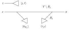
Set \(d_j=\dim \widetilde S_j\) and choose an orthonormal basis \((v_{j\ell })_{0\leq \ell {\lt}d_j}\) of each \(\widetilde S_j\). Define the tag set \(T=\{ (j,\ell ):0\leq j{\lt}n,\ 0\leq \ell {\lt}d_j\} \) and the tag space \(\mathcal J=\mathbb {C}^T\). The encoding \(K\colon \mathcal H_V\to \mathcal J\otimes \mathcal H_V\) is
In particular, the output retains one site register at every site. For input and output configurations \(y,x\in \prod _{v\in V}A_v\), its matrix coefficient is
The reset region in this formula is \(R_j\), determined by the tag. At a fixed tag \(t=(j,\ell )\), the following tensor product depicts its summand.
Identifying coordinate vectors with their Euclidean Hilbert space preserves the dimension of every inside subspace. The tag dimension satisfies
The tags form a disjoint union of sets of cardinality \(d_j\). Sum the inside-dimension inequalities \(\dim \widetilde S_j\leq \dim S_j\).
The encoding has Gram operator
Orthogonality of the tag vectors removes all products between distinct summands of (33). For each remaining summand, \(\langle 0_{R_j} | 0_{R_j} \rangle =1\), so its Gram operator is \(|v_{j\ell }\rangle \! \langle v_{j\ell }|\otimes I_{V\setminus R_j}\). Summing over the orthonormal basis of \(\widetilde S_j\) gives \(P_{\widetilde S_j}\otimes I_{V\setminus R_j}\). Theorem 39.1.7 identifies the sum over \(j\) with \(P_{\mathcal E}\).
For every \(\psi \in \mathcal H_V\),
Thus \(\| K\| \leq 1\).
Since \(P_{\mathcal E}\) is an orthogonal projector, the \(C^*\)-identity gives \(\| K\| ^2=\| K^\dagger K\| =\| P_{\mathcal E}\| \leq 1\). Also,
Taking nonnegative square roots gives the norm equality. The operator-norm bound gives \(\| K\psi \| \leq \| K\| \| \psi \| \leq \| \psi \| \).
For the encoding \(K\) of Definition 39.6.3, every \(\psi \in \mathcal E\) satisfies \(\| K\psi \| =\| \psi \| \). This follows from the Gram identity in the one-hole encoding construction.
Since \(\psi \in \mathcal E\), its orthogonal projection satisfies \(P_{\mathcal E}\psi =\psi \). Hence \(\| K\psi \| =\| P_{\mathcal E}\psi \| =\| \psi \| \) by Theorem 39.6.6.
With a singleton tag set \(\{ \ast \} \), define \(K_{\mathrm{id}}\psi =|\ast \rangle \otimes \psi \). This is the encoding used when an outer square has empty physical sample.
The identity encoding satisfies \(K_{\mathrm{id}}^\dagger K_{\mathrm{id}}=I\). For every \(\psi \in \mathcal H_V\), \(\| K_{\mathrm{id}}\psi \| =\| \psi \| \).
The sum over the singleton tag has one term, and the site matrix is \(I\). Thus the Gram matrix is \(I^\dagger I=I\). Equality of Gram matrices gives equality of the vector norms.
If \(n=0\) or every \(S_j=0\), then \(T\) is empty and \(K=0\).
An empty family has no branch index. If every \(S_j=0\), the tag dimension bound gives \(|T|\leq \sum _{j{\lt}n}\dim (0)=0\). Hence \(T\) is empty. In either case there are no tag coordinates, so the matrix is zero.
If \(n=0\), the tag set \(T\) is empty and \(K=0\); also \(\mathcal E=0\), in agreement with (38). More generally, a zero-dimensional projected image contributes no tags. For an empty region \(R_j\), the inside configuration set is a singleton and \(\mathcal H_{R_j}=\mathbb {C}\); the reset condition is automatic and the complement is all of \(V\). The separate choice \(K_{\mathrm{id}}\) has one tag and retains every site configuration.
39.7 Regional embeddings in uniform physical dimension
Let \(V\) be finite, let \(q\in \mathbb {N}\), and set \(A_q=\{ 0,\ldots ,q-1\} \), with \(A_0=\varnothing \). For \(S\subseteq V\), write \(X_S=A_q^S\) and \(\mathcal H_S=\mathbb {C}^{X_S}\). Fix a region \(R\subseteq V\), its inclusion \(j_R:R\hookrightarrow V\), and an arbitrary matrix \(H\in \operatorname {End}(\mathcal H_R)\). The restriction map identifies \(X_V\) with \(X_R\times X_{V\setminus R}\); let \(L_R(H)\) denote \(H\otimes I_{V\setminus R}\) in the \(X_V\) coordinates. For a site inclusion \(j\), let \(E_j(H)\) act by \(H\) on its image and by the identity on the remaining sites.
For every \(\sigma ,\tau \in X_V\),
Since \(j_R(R)=R\), agreement outside the image of \(j_R\) is precisely equality of the restrictions to \(V\setminus R\). The complementary identity matrix contributes the Kronecker delta \(\delta _{\sigma |_{V\setminus R},\tau |_{V\setminus R}}\). Multiplying it by \(H_{\sigma |_R,\tau |_R}\) gives (41) for both operators.
Let \(\widetilde X_V=\prod _{v\in V}A_q\) and \(\theta _q:X_V\to \widetilde X_V\) be the bijection \(\theta _q(\sigma )=(\sigma (v))_{v\in V}\). Write \(D_R(H)\) for \(H\otimes I_{V\setminus R}\) after splitting this indexed product into its regional and complementary factors. For every \(\alpha ,\beta \in \widetilde X_V\),
The restrictions of \(\theta _q^{-1}(\alpha )\) and \(\theta _q^{-1}(\beta )\) select the same coordinates as the two indexed product factors. Both sides are \(H\) at the regional coordinates when the complementary coordinates agree, and zero otherwise.
For \(R=\varnothing \), \(X_R\) is a singleton and \(L_\varnothing ([c])=cI\); for \(R=V\), \(L_V(H)=H\); and for \(q=1\), every configuration set is a singleton so \(L_R(H)\) is a scalar multiple of the identity.
Take \(V=\{ 0,1\} \), \(R=\{ 0\} \), \(q=2\), and \(H=\bigl(\begin{smallmatrix} 0 & i \\ 2+i & 0 \end{smallmatrix}\bigr)\). Formula (41) gives \(L_R(H)_{(0,0),(1,0)}=i\), \(L_R(H)_{(1,0),(0,0)}=2+i\), and \(L_R(H)_{(0,0),(1,1)}=0\).
39.8 Finite-domain area laws and polynomial PEPS approximation
An entropy bound for every cut and an approximation of the entire vector are different assertions. The first concerns arbitrary finite induced lattice domains. The second asks for one compatible tensor representation on the original open square. We state the two models separately, following [ 286 , 287 ] .
Let \(\Lambda \subset \mathbb Z^2\) be finite. Join sites at coordinate distance one, and let \(d_\Lambda \) be distance in this induced graph, with value \(+\infty \) between distinct components. For \(X\subseteq \Lambda \) and an integer \(r\ge 0\), the closed graph neighborhood
consists of the sites joined to some site of \(X\) by an induced walk of length at most \(r\). At every site put \(\mathbb C^q\), \(q\ge 1\). In configuration coordinates the physical Hilbert space is
Restriction to \(A\) and \(\Lambda \setminus A\) identifies the configuration set with the product of the two regional configuration sets. The configuration set of a region \(A\) has \(q^{|A|}\) elements. Empty domains, holes, and disconnected components are permitted.
Fix an integer \(R\ge 0\) and \(J{\gt}0\). For each nonempty \(X\subseteq \Lambda \) with \(\operatorname {diam}_{d_\Lambda }X\le R\), assign one Hermitian operator \(h_X\) supported on \(X\), with \(\| h_X\| \le J\). The assigned operator may be zero, and acts as the identity on the complementary tensor factors. Define
The norm is the Euclidean operator norm. Boundary edges are unordered and counted once; empty and full cuts have empty boundary.
A pair has induced distance at most \(R\) if and only if an induced walk of length at most \(R\) joins it. Every singleton is an admissible support at every range, and at range zero the admissible supports are exactly the singletons. Adjacent pairs are admissible at range one. The nearest-neighbor graph on \(\{ 0,\ldots ,w-1\} \times \{ 0,\ldots ,h-1\} \) is the induced graph of that integer rectangle, with the corresponding identification of configurations and range-one pair supports.
The extended graph distance is the least walk length, or infinity when no walk exists. A zero-length walk has equal endpoints. A nonempty support of diameter zero therefore has one element. The coordinate embedding preserves horizontal and vertical nearest neighbors and is bijective onto the integer rectangle. Restricting configurations along this bijection gives the last identification.
For a unit vector \(\Omega \), a real \(E_0\), and \(\Delta {\gt}0\), the eigenvector and full-system projector-gap conditions are
For \(A\subseteq \Lambda \), put
All logarithms are natural, with \(0\log 0=0\). The reduced matrix is Hermitian, including when its spectrum contains zero. No condition is imposed on the gap of a Hamiltonian restricted to a smaller region. The uniform boundary assertion requires a single finite constant for each \(q,R,J,\Delta \), chosen before every domain, Hamiltonian, ground vector, and cut.
Let \(H\) be a complex matrix indexed by a finite set, let \(E_0\) be real, and let \(\Omega \) be a unit vector satisfying (50) and (51) with \(\Delta {\gt}0\). As an elementary consequence of the global gap giving the uniqueness assertion in [ 286 , Proposition 4.5 ] , the eigenspace of \(H\) at \(E_0\) is \(\operatorname {span}_{\mathbb C}\{ \Omega \} \).
For an eigenvector \(\psi \) at \(E_0\), the gap inequality gives \(0\ge \Delta \| \psi -\langle \Omega ,\psi \rangle \Omega \| ^2\). Since \(\Delta {\gt}0\), \(\psi =\langle \Omega ,\psi \rangle \Omega \). Conversely, \(H\Omega =E_0\Omega \) puts every scalar multiple of \(\Omega \) in this eigenspace.
Let \(\Lambda \subset \mathbb Z^2\) be finite, let \(q\ge 0\) be an integer, and let \(\Omega \in \mathcal H_\Lambda \). Under the density and entropy conventions of [ 286 , Section 2 ] , for every \(A\subseteq \Lambda \), the regional reduction defined in Definition 39.8.4 satisfies
If \(\| \Omega \| =1\), then for every \(A\subseteq \Lambda \),
If \(\| \Omega \| =1\), the empty region and the full region also satisfy
No Hamiltonian or spectral-gap hypothesis is required. The identities include empty domains and regions and use the one-dimensional empty tensor product. The site dimension \(q\) may here be zero, in which case \(\mathcal H_\Lambda \) is the zero space for nonempty \(\Lambda \); the standing assumption \(q\ge 1\) of Definition 39.8.1 is not needed.
The pure-state matrix \(|\Omega \rangle \langle \Omega |\) is positive semidefinite. Restriction of configurations to \(A\) and its complement changes only the coordinates, and partial trace preserves positivity and trace. Thus \(\operatorname {Tr}\rho _A=\operatorname {Tr}|\Omega \rangle \langle \Omega | =\| \Omega \| ^2\). For a unit vector, the reduced matrix is positive with trace one. Its eigenvalues lie in \([0,1]\), so each term \(-\lambda \log \lambda \) in its entropy is nonnegative, with \(0\log 0=0\).
For the empty region, the reduced matrix acts on a one-dimensional space. For the full region, write \(\rho _\Lambda =MM^*\) using the coefficient matrix of the vector under the configuration splitting. The complement has one configuration, so \(M\) has one column and \(\rho _\Lambda \) has rank at most one. A positive trace-one matrix of rank at most one has one eigenvalue equal to one and all remaining eigenvalues zero. Its entropy therefore vanishes in both cases.
Let \(\mathcal H=\bigotimes _{v\in V}\mathcal H_v\) be a finite tensor product of finite-dimensional complex Hilbert spaces. Let \(H\) be an operator on \(\mathcal H\) and let \(E_0\in \mathbb {R}\). Suppose that \(\Omega \) is a unit vector and \(\Delta {\gt}0\), with
For a unit vector \(\phi \) and a region \(X\subseteq V\), put \(\rho _X^\phi =\operatorname {Tr}_{V\setminus X}|\phi \rangle \langle \phi |\) and define \(\rho _X^\Omega \) in the same way. As in the gap-to-marginal estimate in the proof of Proposition 4.1,
With \(e=\operatorname {Re}\langle \phi ,H\phi \rangle -E_0\), taking the expectation of (60) in \(\phi \) gives \(1-|\langle \Omega ,\phi \rangle |^2\leq e/\Delta \). Contractivity under partial trace and the trace norm formula for two pure states give
Under the hypotheses of Theorem 39.8.7, suppose in addition that
Then, for every region \(X\subseteq V\),
Since \(\Delta {\gt}0\), the quotient of the excess energy by \(\Delta \) is at most \(1/1024\). Theorem 39.8.7 bounds the full trace norm by \(2\sqrt{1/1024}=1/16\).
In Theorem 1.1 of [ 286 ] , for fixed integers \(q\ge 1\), \(R\ge 0\) and reals \(J,\Delta {\gt}0\), there is a finite constant \(C=C(q,R,J,\Delta )\) such that every finite induced domain with the above interaction bounds and a unique unit ground vector, up to phase, satisfying the full-system projector gap obeys \(S_\Omega (A)\le C|\partial _\Lambda A|\) for every \(A\subseteq \Lambda \). The same constant applies to all domains, interaction families, and cuts.
Theorem 44.10.7 has the same hypotheses and gives the bound with \(C=C_{\rm AL}(q,R,J,\Delta )\). That constant is assembled along the following argument.
For disjoint \(B,C\subseteq \Lambda \) write \(I_\Omega (B:C)=S_\Omega (B)+S_\Omega (C)-S_\Omega (B\cup C)\), and let \(Z\) be the set of endpoints of the edges in \(\partial _\Lambda A\). Empty and full cuts have zero entropy, and so does every cut with \(\partial _\Lambda A=\varnothing \). Put \(b=|\partial _\Lambda A|{\gt}0\).
The global gap first gives an exponent below volume: for a box \(Q\) of side at most \(r\), sufficiently far from \(Z\),
Spectral filtering replaces \(H\) by positive quasi-local constraints that annihilate \(\Omega \) and keep a global gap. A replica argument then compares two bounds on a filtered norm while a finite randomized scan moves the partition through a collar. Repeating the comparison improves the exponent in (65) and gives, for a template \(T\) at scale \(n\) and \(L_n=\lfloor n^{1-\varepsilon }\rfloor \),
Here \(\varepsilon \), \(\alpha \) and \(\beta \) are the exponents of Theorem 39.8.41. Products of the positive constraints amplify this bound. For every \(M\ge 1\) there is a radius \(r\le C_Mn^{(1-\varepsilon )/\alpha }\) with \(L_n+2r=o(n^\beta )\) such that
The planar construction partitions \(A\) into a residual set \(D\) and an ordered family of pieces \(X_i\subseteq A\cap T_i\) with labels \(f_i\in \{ 0,1\} \), templates \(T_i\) at scales \(n_i\), and
Put \(S_i=A\cap (T_i)_{L_{n_i}}\) and \(J_i=(\Lambda \setminus A)\cup \bigcup _{j{\lt}i,\, f_j=f_i}X_j\), and let \(r_i\) be the radius in (67) at scale \(n_i\), with the scale threshold large enough that \(L_{n_i}+2r_i{\lt}n_i^\beta \). A walk of length at most \(2r_i\) starting in \(S_i\) stays within ambient distance \(n_i^\beta \) of \(T_i\). By (69) it meets no earlier piece of the same family, and it cannot leave \(A\), since its first step out of \(A\) would end at a point of \(Z\). Hence \(J_i\cap N_{2r_i}^\Lambda (S_i)=\varnothing \). With \(M=100\), (67) and monotonicity of mutual information give
For one family \(f\), with \(A_f=\bigcup _{f_i=f}X_i\) and \(E_f=\sum _{f_i=f}\eta _i\), the chain rule, purity and subadditivity give
Adding (71) for \(f=0\) and \(f=1\) cancels every piece entropy. With (68),
Every threshold and constant above depends only on \(q,R,J,\Delta \), and is chosen before the domain and the cut.
On the original open \(L\times L\) graph, let
where terms are supported on their designated sites or edges, and only the total \(H\) is assumed Hermitian. For a unit vector \(\Omega \), a real \(E_0\), and \(\Delta {\gt}0\), the gapped ground-vector condition for this \(H\) is
A PEPS approximation with parameters \(C,c\) is a tensor family on those same edges with positive dimensions \(D_e\) satisfying \(D_e\le CL^c\) for every edge \(e\), and a nonzero contracted vector \(\Phi \) such that, for some \(\theta \in \mathbb R\),
The norm in (77) is the Euclidean norm of the entire vector. The local tensor maps need not be isometries and the bond dimensions need not be equal. The uniform approximation assertion requires \(C,c{\gt}0\) to be chosen for fixed \(q\ge 2\), \(J,\Delta {\gt}0\) before all \(L\ge 2\), Hamiltonians, and ground vectors.
For vectors \(u,v\) in a complex normed space, the function \(\theta \mapsto \| u-e^{i\theta }v\| \) attains its minimum over \(\mathbb R\). Consequently a bound \(\varepsilon \) holds at some phase if and only if
and (77) holds for some \(\theta \) if and only if it holds with the minimum over \(\theta \), as in the printed target error.
The function is continuous and \(2\pi \)-periodic, so its range is the image of the compact interval \([0,2\pi ]\) and contains its least element. A bound at one phase bounds the infimum, and a bound on the infimum holds at a minimizing phase.
Let \(\mathcal I_L\) be the disjoint union of the vertices of the open square and its forward nearest-neighbor edges. Every undirected edge has exactly one such orientation. The original term indexed by a vertex is its site term, and the term indexed by a forward edge is the term on the corresponding undirected edge.
The support \(S_i\) is \(\{ v\} \) for the vertex label \(i=v\), and \(\{ v,w\} \) for the forward edge label \(i=(v,w)\).
Only the original total Hamiltonian is assumed Hermitian; for the Hermitian replacement of the local terms in [ 287 , Theorem 1.1 ] , for each original term \(A_i\), put
Each \(A_i^{\mathrm h}\) is supported on \(S_i\), is Hermitian, and satisfies \(\| A_i^{\mathrm h}\| \le J\). These conclusions hold for every \(L,q\ge 0\) and every real interaction bound allowed by the original model, including empty grids and zero local dimension.
The supported operators form an algebra closed under adjoints, and hence under real linear combinations. Thus the Hermitian part has the same support. Its adjoint equals itself, and \(\| A_i^{\mathrm h}\| \le \| A_i\| \le J\).
For the original Hermitian Hamiltonian \(H\),
The bijection from forward edges to undirected edges gives \(\sum _i A_i=H\). Taking Hermitian parts commutes with this finite sum, and the Hermitian part of \(H\) is \(H\) itself.
Let \(L\ge 0\) be an integer, and identify the original square-grid sites with \(\Lambda =\{ 0,\ldots ,L-1\} ^2\) by the coordinate bijection \(\sigma \). To view the original square Hamiltonian as a finite-domain interaction family in [ 287 , 286 ] , for an original site or forward-edge label \(i\), define its designated support by
Let \(\sigma \) be the coordinate bijection from the original square-grid sites to \(\Lambda =\{ 0,\ldots ,L-1\} ^2\), with any total order on \(\Lambda \). Let \(e\) send an original site \(v\) to \(\sigma (v)\) and an original forward edge \((v,w)\) to the edge with endpoints \(\sigma (v),\sigma (w)\). For a site or edge label \(j\) in \(\Lambda \), let \(D_j\) be its singleton or two-endpoint support as in [ 287 , Section 1 ] . Then \(X_i=D_{e(i)}\) for every original interaction label \(i\), where \(X_i=\sigma (S_i)\) as in Definition 39.8.17.
For a site label, the image of its singleton is the singleton of its image. For a forward-edge label \((v,w)\), the edge correspondence and graph isomorphism preserve the unordered pair of endpoints, so \(D_{e(i)}=\{ \sigma (v),\sigma (w)\} =\sigma (\{ v,w\} )=X_i\).
For every original site or forward-edge label \(i\), the set \(X_i\) is a nonempty support of induced graph diameter at most one in \(\Lambda \).
If \(i=v\) is a site label, then \(X_i=\{ \sigma (v)\} \) is a singleton, and every singleton is an admissible support at every range. If \(i=(v,w)\) is a forward-edge label, then \(v\) and \(w\) are adjacent in the square grid, so \(X_i=\{ \sigma (v),\sigma (w)\} \) is a pair of adjacent sites of the integer rectangle. Adjacent pairs are admissible at range one.
Distinct original interaction labels have distinct supports \(X_i\).
Site supports are singletons, whereas every edge has two distinct endpoints. Two equal unordered edge supports have equal ordered endpoints or reversed ordered endpoints. The latter case is excluded because both edges have the prescribed forward orientation.
For an integer \(q\ge 0\), let \(U\) be the unitary induced by the site bijection \(\sigma \) on the corresponding configuration spaces. The integer-domain vector corresponding to an original vector \(\Omega \) is \(U\Omega \). The local dimension and every physical tensor factor remain the same.
For every original vector \(\Omega \),
The coordinate identification permutes an orthonormal basis.
The Hermitian part \(A_i^{\mathrm h}\) of every original interaction belongs to the algebra of operators supported on its designated site or edge \(S_i\).
This algebra is closed under adjoints and real linear combinations, so it contains \((A_i+A_i^*)/2\).
Let \(H=\sum _i A_i\) be an original Hermitian square Hamiltonian with interaction bound \(J\in \mathbb R\). At every designated support set
and put \(h_X=0\) at every other admissible range-one support. This defines a Hermitian interaction family on \(\Lambda \), with the same bound \(\| h_X\| \le J\). Indeed, any unused admissible support contains a site \(v\), whose original term gives \(0\le \| A_v\| \le J\). An empty lattice has no admissible supports. Neither a nonempty lattice nor a positive local dimension is required.
The finite-domain interaction has total Hamiltonian
The support map is injective and every unused support contributes zero. Thus the sum is \(\sum _i U A_i^{\mathrm h}U^*\). Conjugation is linear and \(\sum _i A_i^{\mathrm h}=H\).
Let \(H\) be an original square Hamiltonian with interaction bound \(J\in \mathbb R\). Index the sites and unordered nearest-neighbor edges of \(\Lambda \) by \(\mathcal I\), and let \(D_j\) be the singleton or endpoint pair of \(j\). There exist operators \((T_j)_{j\in \mathcal I}\) such that each \(T_j\) is supported on \(D_j\) and
The assertion holds for every side length and local dimension, and for every choice of order on the rectangle sites.
Let \(e\) be the site and edge correspondence, and put \(T_{e(i)}=U A_i^{\mathrm h}U^*\). The support identity gives \(D_{e(i)}=X_i\). The Hermitian part preserves the original support and norm bound, and unitary conjugation preserves Hermiticity and the norm. Finally, the bijection \(e\) preserves the finite sum, so \(\sum _jT_j=U(\sum _i A_i^{\mathrm h})U^*=UHU^*=H_{\mathrm{int}}\).
Let \(E_0,\Delta \in \mathbb R\). If an original unit vector \(\Omega \) satisfies
then \(U\Omega \) is a unit vector satisfying
The conclusion holds for any real lower-gap parameter \(\Delta \). In particular, a positive original full-system gap is preserved.
Conjugating the eigenvector equation and the positive semidefinite gap defect by the unitary \(U\), together with norm preservation, gives both relations.
Let \(\sigma :V\to W\) be a bijection of finite site sets, let \(q\ge 0\), and let \(U_\sigma \) be the unitary that relabels the tensor factors of \((\mathbb C^q)^{\otimes V}\) along \(\sigma \). For every vector \(\Omega \) and every \(A\subseteq V\),
No normalization of \(\Omega \) is required.
Relabeling the sites of \(\sigma (A)\) and of its complement identifies the reduced matrix of \(U_\sigma \Omega \) on \(\sigma (A)\) with the reduced matrix of \(\Omega \) on \(A\), conjugated by a permutation of configurations. A permutation leaves the spectrum, and hence the entropy, unchanged.
For every set \(A\) of sites of the original grid, the number of original edges with exactly one endpoint in \(A\) equals \(|\partial _\Lambda \sigma (A)|\) in the integer rectangle \(\Lambda \).
The coordinate bijection \(\sigma \) is a graph isomorphism onto the induced graph of \(\Lambda \). It therefore maps the crossing edges of \(A\) bijectively onto those of \(\sigma (A)\).
The square-grid entropy area law is the assertion that for every integer \(q\ge 2\) and all reals \(J,\Delta {\gt}0\) there is a constant \(C_A=C_A(q,J,\Delta )\ge 0\) with the following property. For every \(L\), every Hamiltonian of the original model with interaction bound \(J\), and every unit vector \(\Omega \) and real \(E_0\) satisfying \(H\Omega =E_0\Omega \) and \(H-E_0I\ge \Delta (I-|\Omega \rangle \langle \Omega |)\), every set \(A\) of sites of the grid satisfies
where \(\partial _\Lambda A\) is the set of grid edges with exactly one endpoint in \(A\). The constant is chosen before \(L\), \(H\), \(\Omega \) and \(A\).
Let \(q\) be an integer, \(C_A\) a real number, and fix a family of states, consisting for each \(L\) of some vectors on the grid of side \(L\) with local dimension \(q\). The square-grid entropy area law holds for the family with constant \(C_A\) if \(C_A\ge 0\) and, for every \(L\), every state \(\Omega \) of the family and every set \(A\) of sites, \(S_\Omega (A)\le C_A|\partial _\Lambda A|\). The ground states of the model at \(J\) and \(\Delta \) form the family of unit vectors \(\Omega \) for which some Hamiltonian of the original model with interaction bound \(J\) and some real \(E_0\) satisfy \(H\Omega =E_0\Omega \) and \(H-E_0I\ge \Delta (I-|\Omega \rangle \langle \Omega |)\). The square-grid entropy area law of Definition 39.8.30 says that for \(q\ge 2\) and \(J,\Delta {\gt}0\) some constant \(C_A\) has this property for that family.
If the square-grid entropy area law holds for a family of states with constant \(C_A\), it holds with the same constant for every smaller family.
Every state of the smaller family belongs to the larger one.
Assume the uniform finite-domain area-law assertion: for fixed \(q\ge 1\), \(R\ge 0\) and \(J,\Delta {\gt}0\), one constant \(C(q,R,J,\Delta )\ge 0\) bounds \(S_\Omega (A)\) by \(C|\partial _\Lambda A|\) for every finite induced domain, every interaction family of range \(R\) and bound \(J\), every gapped unit ground vector, and every cut. Then the square-grid entropy area law holds, with \(C_A(q,J,\Delta )=C(q,1,J,\Delta )\).
Since \(q\ge 2\), the assumption applies with \(R=1\). Placing \(H\) on the integer rectangle \(\Lambda \) through its Hermitian interaction parts makes \(U\Omega \) a unit ground vector of the resulting Hamiltonian with the same full-system gap \(\Delta \). Applying the assumed bound to the cut \(\sigma (A)\) then gives the result, since its entropy equals \(S_\Omega (A)\) and its crossing edges correspond bijectively to the original crossing edges of \(A\).
In Theorem 1.1 of [ 287 ] , fix an integer \(q\ge 2\) and reals \(J,\Delta {\gt}0\). There are \(C,c{\gt}0\), depending only on these parameters, such that for every \(L\ge 2\), every Hamiltonian in the preceding model with a unique unit ground vector, up to phase, satisfying (76) has a nonzero PEPS on the original open grid with \(D_e\le CL^c\) for every edge \(e\) and
Theorem 39.10.6 has the same hypotheses and gives the approximation with \(C=C_{\rm PEPS}\) and \(c=c_{\rm PEPS}\). Those constants are assembled along the following argument.
Write \(\Lambda _L\) for the sites of the grid and \(\mathcal H_X\) for the tensor product of the site spaces in \(X\subseteq \Lambda _L\). The physical registers are distributed among parties indexed by dyadic squares, starting from one party holding \(\Omega \) and ending with one party per site. The area-law and collar estimates make the mutual information across tapered buffers smaller than any fixed inverse power of \(L\), which lets an owner split its purification approximately. Near a square of logarithmic size, the ground vector is projected with high accuracy onto a sum of mutually orthogonal subspaces
with nested square samples \(X_j\) and orthonormal vectors \(v_{jk}\in \mathcal H_{X_j}\). Each party takes part in boundedly many operations with other parties during its whole lifetime, and each such operation is a sum of polynomially many products of private contractions and bipartite vectors or covectors.
Telescoping the accumulated errors of these contractions, the final vector \(\Psi \) and the final reference vector \(\Omega \otimes \Xi \) satisfy
Density compression replaces the bipartite resources by polynomial sums of product operators and gives an operator network \(\sigma \) on the party graph with polynomial link dimensions and
If \(\eta {\lt}1\), write \(E=\sigma -|\Omega \rangle \langle \Omega |\) and \(a_z=\langle \Omega |z\rangle \) for product basis vectors \(|z\rangle \). Since \(\sum _z\| E|z\rangle \| ^2\le \eta ^2\) and \(\sum _z|a_z|^2=1\), some \(z\) has \(a_z\ne 0\) and \(\| E|z\rangle \| \le \eta |a_z|\). The column \(v=\sigma |z\rangle \) is then nonzero, has the same virtual dimensions, and satisfies
Routing each link horizontally and then vertically through the anchors of the dyadic blocks has edge congestion at most a constant \(\chi \), also after folding the padded grid into the \(L\times L\) grid. If every link has dimension at most \(C_1L^k\), grouping the links crossing each grid edge gives
For \(L\ge L_0\) the error \(2CL^{-5}\) is at most \(L^{-1}\), so (84) gives (79). Each of the finitely many sizes \(2\le L{\lt}L_0\) has an exact representation with bond dimensions bounded independently of the Hamiltonian, which is absorbed by enlarging the prefactor in (85).
Following Definition 9.3 of [ 286 ] , fix \(D_0{\gt}0\) and a sufficiently large positive numerical constant \(C_{\rm tpl}\) before choosing templates. A template with positive integer parameters \(n,s_0\) is a nonempty finite \(T\subset \mathbb Z^2\) with
Each \(P_a\) is a closed convex rectangle or triangle of sup-norm diameter at most \(s_0\), with side slopes in \(\{ 0,\infty ,1,-1\} \). Triangles have noncollinear vertices and rectangles have nonzero sides; this ordinary reading of the source’s polygons is recorded in [ 85 ] . The union may be disconnected. Geometric estimates require a uniform lower bound on \(C_{\rm tpl}\), chosen independently of the template. Separation from a fixed cut set \(Z\) means \(\operatorname {dist}_\infty (T,Z){\gt}4D_0s_0\). For the fixed cut \(A\subseteq \Lambda \) of (49), put
In particular, \(T_0=T\). These are ambient dilations, not the induced-graph neighborhoods (45).
Let \(C_{\rm tpl}\ge 1\) and \(C_{\rm tpl}(s_0+1)\le n\). An integer rectangle \(Q=([x_0,x_1]\times [y_0,y_1])\cap \mathbb Z^2\) with at most \(s_0\) sites along each axis, including a thin rectangle of one row or one column, defines the template with the single piece \(P=[x_0,x_1+\tfrac 12]\times [y_0,y_1+\tfrac 12]\).
For templates \(T\) and \(T'\) with parameters \((n,s_0)\) and \(N_0\) and \(N_0'\) pieces, with \(C_{\rm tpl}(N_0+N_0')(s_0+1)\le n\) and \(\operatorname {diam}_\infty (T\cup T')\le n\), the union template \(T\cup T'\) has the pieces of \(T\) followed by those of \(T'\). The union need not be connected.
For \(C_{\rm tpl}\ge 0\), the template obtained from \(T\) by deleting the pieces with \(P_a\cap \mathbb Z^2=\varnothing \) has the same point set.
The piece \(P\) of a rectangle template is nondegenerate with horizontal and vertical sides, and \(P\cap \mathbb Z^2=Q\), so the rectangle template is \(Q\) with one piece. The union template has point set \(T\cup T'\) and \(N_0+N_0'\) pieces, and omitting empty pieces keeps the point set. If every endpoint of a crossing edge of the cut has sup-norm distance more than \(D|Q|\) from \(Q\), where \(|Q|\) is the larger side, and \(4D_0s_0\le D|Q|\), then the rectangle template is separated from the cut. After empty pieces are omitted, every sampled piece is nonempty and the number of pieces does not increase.
The sup-norm diameter of \(P\) is at most \(|Q|-\tfrac 12\le s_0\), and an integer \(a\) satisfies \(a\le b+\tfrac 12\) exactly when \(a\le b\). The diameter of \(Q\) is less than \(s_0\le n\). The clearance assumption gives \(\operatorname {dist}_\infty (Q,Z){\gt}D|Q|\ge 4D_0s_0\). At least one piece of a template is nonempty because the template is nonempty, and decreasing \(N_0\) preserves \(C_{\rm tpl}N_0(s_0+1)\le n\) when \(C_{\rm tpl}\ge 0\).
A finite region \(A\) is partitioned into a residual set \(D\) and pairwise disjoint pieces \(X_i\). Each piece has a family label in \(\{ 0,1\} \), and one finite order induces the order within each family. For a piece \(X_i\) in family \(f\), the earlier same-family region is \(\bigcup _{j{\lt}i,\, f(j)=f}X_j\). No size, separation, or information bound is assumed in this definition.
Let \(A\subseteq V\) be finite, with an ordered two-family partition whose residual is \(D\) and pieces \(P_i\). If \(W\) is finite and \(f:W\to V\), then \(f^{-1}(A)\) has the partition with residual \(f^{-1}(D)\) and pieces \(f^{-1}(P_i)\), retaining the same labels, families and order. Inverse images commute with the union of all earlier pieces in a given family. If \(f\) is injective, the residual cardinality does not increase.
Inverse images preserve disjointness and unions. The family and order conditions concern only the retained labels, so they are unchanged. The final cardinality bound follows by restricting the injection \(f\) to the residual set. Empty inverse-image pieces retain their labels.
The final box error exponent is \(e_*=2\cdot 10^{-6}\), and the scanner choices are \((\mu ,\nu ,\ell _{\rm sc},\omega ,\kappa )=(1/4,1/1000,1/100000,1/20000,1/1000000)\). The amplification uses \(\varepsilon =10^{-5}\) and \(\alpha =p/(p+1)\). Set \(\beta =1-2\cdot 10^{-6}\), \(\delta _0=2\cdot 10^{-7}\), \(\zeta =1-\delta _0/2\), \(\rho _0=(1+\beta )/2\), and \(\ell _{\rm geo}=10^{-5}\). Then
The choice \(p=10^6\) also satisfies \(p/(p+1){\gt}1-10^{-6}\). The scanner exponent \(\ell _{\rm sc}\) and the geometric exponent \(\ell _{\rm geo}\) are separate choices, which happen to have the same value.
Substituting the stated rational values and comparing integers after multiplying by positive denominators shows that each gap is strictly positive.
Fix \(q,R,J,\Delta \) and the template constants \(D_0,C_{\rm tpl}\). For disjoint \(B,C\subseteq \Lambda \) write \(I_\Omega (B:C)=S_\Omega (B)+S_\Omega (C)-S_\Omega (B\cup C)\). The sublinear collar bound of Proposition 9.6 of [ 286 ] for these constants is the assertion that there are \(C\) and \(N\) with the following property. Let \(n\ge N\), let \(\Omega \) be the gapped ground vector of an admissible Hamiltonian on a finite induced domain \(\Lambda \), let \(A\subseteq \Lambda \), and let \(T\) be a template with parameters \((n,s_0)\) separated from the endpoints of the cut edges. Put \(L=\lfloor n^{1-\varepsilon }\rfloor \), \(X=A\cap T\) and \(S_0=A\cap T_L\), and suppose \(L\le s_0\). Then
and each of the cuts \(X\), \(S_0\) and \(S_0\setminus X\) has at most \(Cn\) crossing edges. When this property holds for a given pair \((C,N)\), we say that the sublinear collar bound holds with constant \(C\) and threshold \(N\); the sublinear collar bound is the existence of such a pair.
Fix \(q,R,J,\Delta \). The amplification bound of Proposition 10.2 of [ 286 ] is the assertion that for every \(C_0{\gt}0\) and every integer \(M\ge 1\) there are \(C_M\) and \(N\) with the following property. Let \(n\ge \max (2,N)\), let \(\Omega \) be the gapped ground vector of an admissible Hamiltonian on a finite induced domain \(\Lambda \), let \(A\subseteq \Lambda \) and let \(T\subset \mathbb Z^2\) be finite. Put \(L=\lfloor n^{1-\varepsilon }\rfloor \), \(X=A\cap T\), \(S_0=A\cap T_L\) and \(Y=S_0\setminus X\). Suppose that \(|S_0|\le C_0n^2\), that each of the cuts \(X\), \(Y\), \(S_0\) has at most \(C_0n\) crossing edges, and that \(I_\Omega (X:\Lambda \setminus S_0)\le C_0n^{1-\varepsilon }\). Then there is an integer \(r\le C_Mn^{(1-\varepsilon )/\alpha }\) such that
If in addition \(\operatorname {dist}_\infty (T,Z){\gt}L+n^\beta \), where \(Z\) is the set of endpoints of the cut edges, then \(N_{2r}^\Lambda (S_0)\subseteq A\); its further assertion \(L+2r=o(n^\beta )\) follows from the radius bound by Theorem 42.7.3. When this property holds for given \(C_0\), \(M\) and a given pair \((C_M,N)\), we say that the amplification bound holds at \((C_0,M)\) with constant \(C_M\) and threshold \(N\).
Fix the template constants \(D_0,C_{\rm tpl}\). The two-family decomposition of Proposition 11.2 of [ 286 ] for these constants is the assertion that for every \(n_*\ge 1\) there is \(C\) with the following property. For every finite induced domain \(\Lambda \) and every \(A\subseteq \Lambda \) with \(b=|\partial _\Lambda A|{\gt}0\), with \(Z\) the set of endpoints of the cut edges, there is an ordered two-family partition of \(A\) into a residual set \(D\) and nonempty pieces \(X_i\) with labels \(f_i\), together with templates \(T_i\) with parameters \((n_i,s_i)\), such that \(|D|\le Cb\), \(X_i\subseteq A\cap T_i\), each \(T_i\) is separated from \(Z\), \(\lfloor n_i^{1-\ell _{\rm geo}}\rfloor \le s_i\), \(n_i\ge n_*\),
and \(\sum _in_i^{-100}\le Cb\).
At every generation of the repair construction, an identifier of birth rank zero other than the dummy is a retained primary of a layer \(k\ge k_0\), and its characteristic length is \(r=2^k\). Its closed birth region lies at distance at least \(\min (t_k,r/2)\) from the closed birth region of every other identifier of birth rank zero with the same label. For every \(C_P{\gt}0\) there is a constant \(M\), chosen before the origin, the domain, the cut and the construction parameters, such that every finite set of such identifiers satisfies
where \(C\) is the layer width.
The identifier is the image of a unique original primary, and retention preserves its birth region, its label and its characteristic length. Equal labels of primaries mean equal layer parity, so the separation of primary birth regions of the same parity applies. For the sum, distinct identifiers come from distinct primaries; grouping them by layer bounds the sum by the weighted count of primaries over finitely many layers.
At a generation \(N\) of the repair construction without marks, suppose that the marks of the generations before \(N\) number at most \(M(2C+1)^2|\partial _\Lambda A|\) in total. Then the sites of \(A\) in the dummy region or in a terminal square number at most
At an empty generation every terminal square was removed at an earlier generation. The two terms bound the dummy sites and the sites of the terminal squares of those generations.
The constant \(C_{\rm tpl}\) enters a template only through \(C_{\rm tpl}N_0(s_0+1)\le n\), whose other factors are nonnegative, so a template for \(\max (C_{\rm tpl},1)\) is a template for \(C_{\rm tpl}\). We may therefore assume \(C_{\rm tpl}\ge 1\). Fix \(n_*\ge 1\). The constants are chosen in the order of the source. First take the template coefficients \(C_P\) and \(C_B\) for \(C_{\rm tpl}\), the isolation constant \(a_0=1/4\), and the separation constant \(c_1\). Next take \(u_*\) so large that every \(u\ge u_*\) satisfies \(2\lceil C_Bu\rceil ^\beta {\lt}c_1u^{\rho _0}\), \(\lfloor \lceil C_Bu\rceil ^{1-\ell _{\rm geo}}\rfloor \le u\) and \(C_Bu\ge n_*\), and take the stopping scale \(S_*\ge \max (u_*,2)\) above the thresholds of the template, isolation and separation estimates. Then take the layer width \(C{\gt}4D_0\), and finally \(k_0\) above the thresholds of the templates, of the isolation hypotheses, of birth separation, of the lower bound \(u\ge u_*\) for the characteristic lengths of positive birth rank, and of the primary scale limits with factor \(1/8\) and \(n_*\).
Let \(\Lambda \) and \(A\) with \(b=|\partial _\Lambda A|{\gt}0\) be given, and run the repair construction at the prescribed origin. It reaches a generation without marks. The non-dummy identifiers whose current regions meet \(A\), ordered by nondecreasing birth rank, give the pieces \(X_i\) and their labels; the residual set \(D\) consists of the sites in the dummy region or in a terminal square. Each piece lies in the lattice sample of the closed birth region of its identifier, and that sample is the point set of a template with both endpoint clearances. Its scanner scale is \(n=\lceil C_P\, r^{1+2\delta _0}\rceil \) for a primary of side \(r=2^k\) and \(n=\lceil C_Bu\rceil \) for an identifier of positive birth rank and characteristic length \(u\). The primary scale limits and the choice of \(u_*\) give \(\lfloor n^{1-\ell _{\rm geo}}\rfloor \le s\) and \(n\ge n_*\).
For the ordered clearance, let \(j{\lt}i\) have the same label. Then the birth rank of \(X_j\) is at most that of \(X_i\). If \(X_i\) is a primary of layer \(k\), so is \(X_j\), and the closed birth regions are at distance at least \(\min (t_k,2^{k-1})\), which exceeds \(2n^\beta \) by the primary scale limits. Otherwise birth separation at a common generation, with final regions equal to current regions at an empty generation, gives distance at least \(c_1u^{\rho _0}{\gt}2\lceil C_Bu\rceil ^\beta \).
Finally, \(|D|\le Cb\) by Lemma 39.8.46 and the total mark count. The sum \(\sum _in_i^{-100}\) splits into the primaries, bounded by Lemma 39.8.45, and the retained identifiers of positive birth rank, bounded by their error sum.
Suppose that for all \(q\ge 1\), \(R\ge 0\) and \(J,\Delta {\gt}0\) there are template constants \(D_0,C_{\rm tpl}\) for which the sublinear collar bound and the two-family decomposition hold, and that the amplification bound holds for all such \(q,R,J,\Delta \). Then the conclusion of Theorem 39.8.9 holds, proving Theorem 1.1 of [ 286 ] conditionally on the three propositions: for each \(q,R,J,\Delta \) there is one \(C\ge 0\) such that \(S_\Omega (A)\le C|\partial _\Lambda A|\) for every finite induced domain, every admissible Hamiltonian with a gapped ground vector \(\Omega \), and every \(A\subseteq \Lambda \).
Fix \(q,R,J,\Delta \) and take template constants \(D_0,C_{\rm tpl}\) with the collar bound and the two-family decomposition. Choose the collar constant \(C_1\) and threshold \(N_1\), then the amplification constant \(C_2\) and threshold \(N_2\) at the input constant \(\max \{ C_1,1\} \) and the order \(100\), and then a two-family constant \(C_3\) at the lower scale \(n_*(N_1,N_2,C_2)\ge 2\). Theorem 44.10.2 gives the bound with the constant \(C(q,C_2,C_3)\ge 0\), which is chosen before the domain and the cut.
The proof of Proposition 9.6 of [ 286 ] combines the scanner estimates with three steps that use no estimate of the scan: an exact entropy identity at each leaf, the transfer from the truncated to the original ground state, and the cut and size assertions of the proposition. The results below prove these steps. Theorem 39.9.9 combines them with the physical scanner estimates to prove the information inequality.
Let \(\psi \) be a vector of a finite tensor product over a site set \(V\), and let \(X,U,Y,W\subseteq V\). Put
Let \(X,U,Y,W\) be pairwise disjoint sets covering \(V\). As in the leaf entropy identity and the lower bound after the leaf average in the proof of Proposition 9.6 of [ 286 ] , for every vector \(\psi \),
If a set \(F\) lies in \(W\), then \(2I(X:F)\le 2S(X)+g_{\rm pre}-g_{\rm post}\). Consequently, for finitely many leaves with weights \(p_i\ge 0\) summing to one, each with its own partition \(X,U_i,Y_i,W_i\) of \(V\) and with \(F\subseteq W_i\) for every \(i\),
Purity gives \(S(X\cup W)=S(U\cup Y)\), \(S(X\cup Y\cup W)=S(U)\) and \(S(Y\cup W)=S(X\cup U)\), and the identity follows by expanding both mutual informations. Strong subadditivity makes mutual information monotone in each argument, and both \(W\) and \(Y\cup W\) contain \(F\). Multiplying the bound at each leaf by \(p_i\) and summing gives the average inequality.
Let \(\Omega ,\widetilde\Omega \) be unit vectors at trace distance \(\delta \), and let \(X,J\) be disjoint. Then
In particular, if \(\delta \le C_1n^{-500}\) and \(\log \dim \mathcal H_X\le C_2n^2\) for an integer \(n\ge 1\), then \(I_\Omega (X:J)\le I_{\widetilde\Omega }(X:J)+8\sqrt{C_1}(1+C_2)n^{-248}\). The dimension of \(J\) does not enter.
Let \(T\) be a template with parameters \((n,s_0)\) separated from the cut, with \(C_{\rm tpl}\ge 24\) and \(D_0\ge 1\), and let \(L\le s_0\). Put \(X=A\cap T\) and \(S_0=A\cap T_L\). Then the cuts of \(X\) and \(S_0\) have at most \(4n\) edges, the cut of \(S_0\setminus X\) has at most \(8n\) edges, and \(|S_0|\le 10n^2\).
The cut bounds are those of Theorem 41.12.1.3 with \(j=L\), since \(S_0\setminus X=A\cap (T_L\setminus T)\). The set \(S_0\) lies in \(T_L\), and \(|T_L|\le |T|+nL\le 9ns_0+nL\) by the area and depth-layer bounds. The scale condition \(C_{\rm tpl}N_0(s_0+1)\le n\) gives \(L\le s_0\le n\).
Let \(C_{\rm tpl}\ge 24\) and \(D_0\ge 1\). Suppose there are \(C\) and \(N\) such that, in the setting of Definition 39.8.42, \(I_\Omega (X:\Lambda \setminus S_0)\le Cn^{1-\varepsilon }\) whenever \(n\ge N\). Then the sublinear collar bound holds for \(D_0,C_{\rm tpl}\), reducing Proposition 9.6 of [ 286 ] to its information inequality.
Taking the constant \(\max (C,10)\) combines the assumed information inequality with the remaining assertions of Theorem 39.8.52.
39.9 Companion area-law inputs
The proof of Theorem 39.8.35 uses several results of the area-law companion [ 286 ] , which are listed in [ 287 , Appendix A ] . All of them concern the original ground vector \(\Omega \) of the full system; no subregion is assigned a gap of its own. The remarks below compare each listed result with the statement of this chapter that expresses it. No statement below adds a hypothesis to the printed one. The appendix also records that the companion takes its replica limit at each fixed finite instance; this concerns the companion’s proof of the collar bound, and the statements below concern only the original one-copy state.
The companion allows every finite induced domain \(\Gamma \subset \mathbb Z^2\) with local dimension \(q\), and one Hermitian term \(h_X\) with \(\| h_X\| \le J\) for each nonempty support \(X\) of induced-graph diameter at most \(R\). It assumes a unit ground vector \(\Omega \) with \(H-E_0I\ge \Delta (I-|\Omega \rangle \langle \Omega |)\), and its entropies use natural logarithms [ 287 , Appendix A ] . Definitions 39.8.1, 39.8.2 and 39.8.4 state exactly this model: zero terms are allowed, the domain need not be connected, norms are operator norms, and entropy is the von Neumann entropy with natural logarithms. Uniqueness of the ground vector up to phase is not a separate hypothesis. It follows from the gap inequality by Theorem 39.8.5.
Theorem 1.1 and Corollary 1.2 of [ 286 ] give Proposition 2.1 of [ 287 ] , with \(\Gamma \) the \(L\times L\) grid and \(R=1\). Theorem 39.8.9 states the uniform finite-domain area law with the printed quantifiers: one constant \(C(q,R,J,\Delta )\) serves every domain, interaction family and cut. Theorem 42.10.14 derives it from Propositions 9.6 and 11.2 of [ 286 ] . The collar proposition is Theorem 39.9.9; amplification is Theorem 42.10.12. The site and edge terms of the original model need not be Hermitian individually. Replacing each by its Hermitian part keeps its support and norm bound and leaves the total Hamiltonian unchanged (Theorem 39.8.16). Theorem 39.8.34 then specializes the uniform area law to the square at range one with \(C_A(q,J,\Delta )=C(q,1,J,\Delta )\), and Theorem 39.11.9 gives the same conclusion through the rectangle corollary, giving Proposition 2.1 (Theorem 39.8.33) from the uniform area law.
For every integer \(k\ge 1\) and \(\alpha =k/(k+1)\), the appendix uses positive contractions \(k_i\) at the original anchors, of uniformly bounded anchor multiplicity, with \(k_i\Omega =0\), \(\sum _ik_i\ge c_*^{-1}(H-E_0I)\ge (\Delta /c_*)(I-|\Omega \rangle \langle \Omega |)\) and \(\| k_i-\mathbb E_{N_r(a_i)}k_i\| \le Ce^{-cr^\alpha }\) for every integer \(r\ge 0\) [ 286 , Proposition 4.3 ] . Theorem 43.2.2 states this for every choice of anchors \(a_i\in X_i\), with constants depending only on \(k,R,J,\Delta \) and under the weaker condition \(J\ge 0\). Its tail estimate is stated for conditional expectation onto every induced-graph ball. At most \(2^{2R(R+1)}\) labels share an anchor, by Theorem 43.2.1.
Definition 39.8.36 states the templates of [ 286 , Definition 9.3 ] with the printed conditions \(n\ge C_{\rm tpl}N_0(s_0+1)\), \(\operatorname {diam}_\infty T\le n\) and \(\operatorname {dist}_\infty (T,Z_A){\gt}4D_0s_0\); the polygons are read as nondegenerate [ 85 ] . Definition 39.8.42 states the sublinear collar bound, Proposition 9.6 of [ 286 ] , with \(\varepsilon =10^{-5}\), \(\ell =\lfloor n^{1-\varepsilon }\rfloor \le s_0\), \(X=A\cap T\) and \(S_0=A\cap T_\ell \): at every scale beyond a uniform threshold, \(I_\Omega (X:\Gamma \setminus S_0)\le Cn^{1-\varepsilon }\), \(|S_0|\le Cn^2\), and each of \(X\), \(S_0\setminus X\) and \(S_0\) has at most \(Cn\) crossing edges. For \(C_{\rm tpl}\ge 24\) and \(D_0\ge 1\), which the standing choices of a large \(C_{\rm tpl}\) and of \(D_0{\gt}2R+10\) ensure, the size and crossing-edge assertions hold for every separated template (Theorem 39.8.52), so Theorem 39.8.53 reduces the proposition to the information inequality alone. This inequality, together with the size and crossing-edge bounds, is Theorem 39.9.9.
Definition 39.8.43 states Proposition 10.2 of [ 286 ] as printed in the appendix: from the three collar bounds with a common constant \(C_0\), for every integer \(M\ge 1\) and every sufficiently large \(n\), a radius \(r\le C_Mn^{(1-\varepsilon )/\alpha }\) with \(I_\Omega (X':E)\le C_Mn^{-M}\) for every \(X'\subseteq X\) and every \(E\subseteq \Gamma \setminus N_{2r}(S_0)\), and \(N_{2r}(S_0)\subseteq A\) when \(\operatorname {dist}_\infty (T,Z_A){\gt}\ell +n^{\beta _0}\), where \(\beta _0=1-2\cdot 10^{-6}\). The exponent \(\alpha =p/(p+1)\) is fixed with \(p=10^6\), an admissible choice for the requirement \(\alpha {\gt}1-10^{-6}\). The remaining assertion \(\ell +2r=o(n^{\beta _0})\) follows from the radius bound (Theorem 42.7.3). The bound holds for every gap \(\Delta {\gt}0\) (Theorem 42.10.12). Its application in [ 287 , Proposition 3.1 ] , with \(A=\Gamma \) and \(M=1\), is Theorem 42.11.8, which derives it from the sublinear collar bound. Theorem 42.11.4 establishes the original-gap conclusion using the physical collar theorem.
For a pure state and an ordered partition \(A=D\mathbin {\dot\cup }\bigcup _iX_i\) into two labelled families, the bounds \(I(X_i:A^c\cup \bigcup _{j{\lt}i,\, f_j=f_i}X_j)\le \delta _i\) give \(S(A)\le S(D)+\frac12\sum _i\delta _i\) [ 286 , Lemma 11.1 ] . Theorem 42.1.1 states this for a unit vector in any finite tensor product of finite-dimensional spaces.
Definition 39.8.44 states Proposition 11.2 of [ 286 ] as printed in the appendix: for every cut with \(b=|\partial _\Gamma A|{\gt}0\) and every lower scale \(n_*\), a partition with \(|D|\le Cb\), nonempty pieces \(X_i\subseteq A\cap T_i\), separated templates with \(n_i\ge n_*\) and \(\lfloor n_i^{1-\varepsilon }\rfloor \le s_i\), both clearances \(2n_i^{\beta _0}\), and \(\sum _in_i^{-100}\le Cb\), with \(C\) depending only on \(n_*\) and the template constants. Theorem 39.8.47 proves it for all real \(D_0\) and \(C_{\rm tpl}\).
The appendix states that [ 287 , Lemma 3.2 ] adapts the ordering of Lemma 11.1 of [ 286 ] to a cell with arbitrary exterior conditioning, and that this adaptation is proved in the approximation article rather than imported. Its entropy estimate is Theorem 42.2.1, and its two-family partition of a cell is Theorem 42.2.10. Neither obtains a conditional information bound by conditioning a mutual-information inequality. Together these give the cell estimate of Theorem 39.5.1.
In [ 286 , Proposition 9.6 ] , fix \(q,R\in \mathbb N\) with \(q\geq 1\), real parameters \(J\geq 0\) and \(\Delta {\gt}0\), and real template constants \(D_0{\gt}2R+10\) and \(C_{\mathrm{tpl}}\geq 24\). There are \(C\in \mathbb R\) and \(N\in \mathbb N\), chosen before all the following finite data. Let \(\Lambda \) be a finite induced square-lattice domain, let \(H\) be an admissible Hamiltonian with parameters \((q,R,J)\), and let \(\Omega \) be its normalized ground vector at energy \(E_0\) with full-system projector gap \(\Delta \). Let \(A\subseteq \Lambda \) and let \(Z\) be the endpoints of its cut edges. For every template \(T\) with parameters \((C_{\mathrm{tpl}},n,s_0)\) satisfying \(n\geq N\), \(\operatorname {dist}_\infty (T,Z){\gt}4D_0s_0\), and \(L=\lfloor n^{1-1/100000}\rfloor \leq s_0\), put \(X=A\cap T\) and \(S_0=A\cap T_L\). Then
and each of \(X\), \(S_0\), and \(S_0\setminus X\) has at most \(Cn\) crossing edges in \(\Lambda \).
Put \(d=2R+10\). The physical safe-box bound at the integer clearance \(d+1\) gives \(C_b{\gt}0\) at exponent \(1+e_*\), where \(e_*=2\cdot 10^{-6}\). The clearance comparison gives
at every positive integer scale. The conditional template information theorem at clearance \(d\), which requires only \(d\geq 1\), gives \(C_m{\gt}0\) and a threshold, before all finite instances, for which \(2I_\Omega (X:\Lambda \setminus S_0)\leq C_m n^{1-1/100000}\). The hypothesis \(D_0{\gt}d\) ensures that every template separated at the prescribed real clearance \(D_0\) is also separated at \(d\). The estimate therefore applies to the same original vector and the unchanged regions \(X\) and \(S_0\).
Dividing the information coefficient by two and applying Theorem 39.8.53 shows that the single constant \(\max (C_m/2,10)\) also bounds the three cuts and the collar cardinality, with the same threshold.
This is an auxiliary refinement of Theorem 39.9.9 with two hypotheses that [ 286 , Proposition 9.6 ] does not carry. Fix the data \(q,R,J,\Delta ,D_0,C_{\mathrm{tpl}}\) of that theorem.
Suppose \(C_b\geq 0\) satisfies \(F_{\mathrm{box},2R+11}(r)\leq C_br^{1+e_*}\) for every integer \(r\geq 1\). Then there are truncation and transport constants of the scanner such that the conclusions of Theorem 39.9.9 hold with \(C=\max (C_m/2,10)\), where \(C_m\) is the collar information coefficient at the input \(4C_b+4\log q+1\), and with a threshold \(N\) given by an explicit formula in \(C_b\) and these constants.
Suppose \(C_0\geq 0\) and \(0{\lt}e_0{\lt}1\) satisfy \(F_{\mathrm{box},D}(r)\leq C_0r^{1+e_0}\) for every integer \(D{\gt}2R+10\) and every integer \(r\geq 1\). Then the same holds with \(C_b\) the constant produced by the safe-box bootstrap from \(C_0\) and \(e_0\).
For the first part, the clearance comparison turns the bound at clearance \(2R+11\) into the bound with constant \(4C_b+4\log q+1\) at the integer clearance \(d=2R+10\). The template information theorem at clearance \(d\) gives the information coefficient \(C_m\) and its threshold as formulas, and Theorem 39.8.53 converts them into the constant \(\max (C_m/2,10)\) for all the conclusions. For the second part, the physical safe-box bootstrap of Theorem 44.24.13 gives \(C_b\) from the initial bound, and the first part applies.
Fix the data \(q,R,J,\Delta ,D_0,C_{\mathrm{tpl}}\) of Theorem 39.9.9, and real numbers \(c_0,C_{\rm ent},e_{\rm ent},C_{\rm en},e_{\rm en}\) with \(c_0{\gt}0\) for which the common step-error bound of Theorem 43.3.1.15 holds. Let \(C_{\rm box}\) be the safe-box constant of the bootstrap of Theorem 44.24.13 started from the explicit initial box estimate, with the truncation constant at the factor \(2\) and these transport constants. Then the conclusions of Theorem 39.9.9 hold with the constant \(C_1\) and the threshold \(N_1\) of the collar bound at \(C_{\rm box}\), the truncation constant at the factor \(10\) and these transport constants.
The bootstrap of Theorem 44.24.13, run from the explicit initial box estimate at the given transport constants, gives \(F_{\mathrm{box},2R+11}(r)\leq C_{\rm box}r^{1+e_*}\) for every integer \(r\geq 1\), with \(C_{\rm box}\geq 0\). The argument of the first part of Theorem 39.9.10 is then run at the same transport constants and the truncation constant at the factor \(10\): the clearance comparison passes to clearance \(2R+10\), the template information theorem gives the information coefficient and its threshold, and Theorem 39.8.53 converts them into \(C_1\) and \(N_1\).
39.10 The constants produced by the proof of the polynomial PEPS approximation
Theorem 1.1 of [ 287 ] asserts that its constants exist. Its proof in Section 8 fixes them in a definite order (07-assembly.tex, lines 179–214). This section writes the constants of the large sizes as functions of three inputs: the constant of the square area law, and the slope and the threshold of Proposition 3.4. Every other choice is a fixed number.
Fix \(q\ge 2\) and a family of unit states, consisting for each side \(L\) of some unit vectors on the square of side \(L\). Let \(\epsilon _0=1/30000\), \(\nu =1/600000000\), \(a_0=1/5000\) and \(b=\max \{ 18,\lceil ((4+8\epsilon _0+2\nu )/\nu +1)^2\rceil \} \). Let \(D\ge 1\) and \(L_{\rm ang}\) be a slope and a threshold at accuracy \(L^{-60}\) for the family, the clearance \(a_0/2\), the diameter ratio \(1\) and at most \(4\) marked points. Let \(C{\gt}0\) and \(c\) be constants with which adaptive patches, in the sense of Proposition 4.1, are supplied on the cell-center sites at the radius constant \(B_0=20D\) and power \(60\), for every state of the family of side \(L\ge 2\). Put \(C'=\lceil C\rceil \), \(c'=\lceil c\rceil \),
Then for every count constant \(C_N\ge 5042\), expansion constant \(C_K\ge G\) and error constant \(C_E\ge \max \{ 10080,2b+1\} \), every \(L\ge 2\) with \(L\ge \lceil \max \{ L_{\rm ang},1\} \rceil \) and every state \(\Omega \) of the family of side \(L\), there is a protocol with the Section 8 bounds of Definition 45.1.1.1 at the constants \(C_N\), \(C_K\), \(C_E\), the bound \(64\cdot 189\), the exponent \(k_K\) and \(2b\) pair effects.
This is the argument of Theorem 45.15.82, with the slope and the patch constants given instead of chosen. The mesh ratio \(\nu \) serves the resizes, the point treatments and the direct repaintings at once, so the constants \(K_0=20\), \(\epsilon _0\), \(\nu \), \(a=a_0/2\), \(D\) and \(B_0=K_0D\) satisfy the conditions of the protocol constants. For \(L\ge \lceil \max \{ L_{\rm ang},1\} \rceil \) the slope applies at side \(L\).
Fix an integer \(q\) and reals \(J,\Delta ,C_A,D,L_{\rm ang}\). Let \(\epsilon _0=1/30000\), \(\nu =1/600000000\), \(b_{\rm prot}=64\cdot 189\) and
Let \(C=\max \{ q^{81},1+10D\} \) and \(c\) be the constants of Definition 45.11.4 at \(B_0=20D\), \(p=60\) and \(C_A\), and let \(G\) and \(k_K\) be as in Theorem 45.1.1.4, with \(C'=\lceil C\rceil \) and \(c'=\lceil c\rceil \). Let \(C_E=\max \{ 10080,2b+1\} \). The link exponent and the link prefactor are
the constants of Definition 45.59.9 and Definition 45.59.12 at \(2b\) pair effects, arity \(b_{\rm prot}\), gate-count exponent \(3\), physical-dimension exponent \(0\), monomial and coefficient-sum exponent \(k_K\) and accuracy \(L^{-5}\). Put
The bond exponent and the bond prefactor for large sizes are
Both are positive. Only \(c_{\rm PEPS}\) depends on \(C_A\); \(C_{\rm large}\) depends on \(q\) and \(D\), and \(L_0\) on \(L_{\rm ang}\) alone. More generally, for a real \(c\) write \(k(c)\) and \(c_{\rm PEPS}(c)=k(c)\chi +1\) for the link and bond exponents obtained in the same way with \(c\) in place of the patch exponent; then \(c_{\rm PEPS}=c_{\rm PEPS}(c(q,J,\Delta ,20D,60,C_A))\), and \(c_{\rm PEPS}(c){\gt}0\).
Fix an integer \(q\ge 2\) and a family of unit vectors on the \(L\times L\) grids. Let \(D\ge 1\) and \(L_{\rm ang}\) be a slope and a threshold at accuracy \(L^{-60}\) for this family, the clearance \(a_0/2\), \(a_0=1/5000\), the diameter ratio \(1\) and at most \(4\) marked points, and let \(c\) be a real such that every member of the family on a grid of side \(L\ge 2\) has adaptive patches on the cell-center sites at \(B_0=20D\), power \(60\), prefactor \(C(q,20D)\) and exponent \(c\). Then every member \(\Omega \) of the family on a grid of side \(L\ge 2\) with \(L\ge L_0\) has a nonzero PEPS \(\Phi \) on the \(L\times L\) grid with \(D_e\le C_{\rm large}L^{c_{\rm PEPS}(c)}\) for every edge \(e\) and
The proof of Theorem 39.8.35 uses the Hamiltonian only through the slope and the patches, so this form applies to any family for which both are available.
Lemma 39.10.1 at \(C_N=5042\), \(C_K=G\) and \(C_E=\max \{ 10080,2b+1\} \) gives the protocol for \(L\ge \lceil \max \{ L_{\rm ang},1\} \rceil \). Compression at accuracy \(L^{-5}\), as in Theorem 45.63.1.6, gives an operator network with error \(C_{\rm net}L^{-5}\), link dimensions at most \(C_1L^{k(c)}\), at most \(b_{\rm prot}\) parties per block, at most \(2b_{\rm prot}(b_{\rm prot}-1)\) links per party and separations at most \(b_{\rm prot}\). For \(L\ge \lceil 2C_{\rm net}\rceil \) the routing argument of Theorem 45.63.1.3 gives bonds at most \(\max \{ C_1,1\} ^\chi L^{k(c)\chi +1}\) and error at most \(L^{-1}\).
Fix an integer \(q\ge 2\) and reals \(J,\Delta {\gt}0\). Assume the square-grid entropy area law for the ground states of the model at \(J\) and \(\Delta \) with constant \(C_A\), and let \(D\ge 1\) and \(L_{\rm ang}\) be a slope and a threshold at accuracy \(L^{-60}\) for these ground states, the clearance \(a_0/2\), \(a_0=1/5000\), the diameter ratio \(1\) and at most \(4\) marked points. Let \(c_{\rm PEPS}\), \(C_{\rm large}\) and \(L_0\) be the constants of Definition 39.10.2. Then for every \(L\ge 2\) with \(L\ge L_0\), every Hamiltonian of the model of Theorem 39.8.35 and every unit ground vector \(\Omega \) with gap \(\Delta \), there is a nonzero PEPS \(\Phi \) on the \(L\times L\) grid with \(D_e\le C_{\rm large}L^{c_{\rm PEPS}}\) for every edge \(e\) and
The area law and the slope are inputs of the proof of Theorem 39.8.35, not hypotheses of that theorem, and the sizes \(L{\lt}L_0\) are not covered here.
By Theorem 45.11.6 the area law supplies adaptive patches at \(B_0=20D\) and power \(60\) with the constants \(C\) and \(c\); moving them to the cell-center sites keeps the constants. The ground states of the model are unit vectors, and Theorem 39.10.3 at this \(c\) gives the approximation, since \(c_{\rm PEPS}=c_{\rm PEPS}(c)\).
Fix an integer \(q\) and reals \(J,\Delta \), and let \(a_0=1/5000\). Let \(C_A=C_{\rm AL}(q,1,J,\Delta )\) be the area-law constant of Definition 44.10.6 at range one. Let \(D=D_{\rm ang}(J,\Delta ,a_0/2,60)\) and \(L_{\rm ang}=L_{\rm ang}(q,J,\Delta ,a_0/2,1,4,60)\) be the angular slope and the angular size threshold of Definition 39.5.3. With \(L_0\), \(c_{\rm PEPS}\) and \(C_{\rm large}\) the constants of Definition 39.10.2 at \(C_A\), \(D\) and \(L_{\rm ang}\), put
Both \(C_{\rm PEPS}\) and \(c_{\rm PEPS}\) are positive, and they depend only on \(q\), \(J\) and \(\Delta \).
Fix an integer \(q\ge 2\) and reals \(J,\Delta {\gt}0\), and let \(C_{\rm PEPS}\) and \(c_{\rm PEPS}\) be the constants of Definition 39.10.5. For every \(L\ge 2\), every Hamiltonian of the model of Theorem 39.8.35 and every unit ground vector \(\Omega \) with gap \(\Delta \), there is a nonzero PEPS \(\Phi \) on the \(L\times L\) grid with \(D_e\le C_{\rm PEPS}L^{c_{\rm PEPS}}\) for every edge \(e\) and
The source theorem asserts only that such constants exist.
By Theorem 44.10.21 the square-grid entropy area law holds with the constant \(C_A\). By Theorem 39.5.4, \(D\) and \(L_{\rm ang}\) are a slope and a threshold at accuracy \(L^{-60}\), and \(D\ge 1\). Then Theorem 39.10.4 gives the approximation with the prefactor \(C_{\rm large}\) for \(L\ge L_0\), and Lemma 45.63.2 extends it to every \(L\ge 2\) with the prefactor \(C_{\rm PEPS}\).
39.11 Rectangular consequences of the uniform entropy bound
Let \(V=\{ 0,\ldots ,w-1\} \times \{ 0,\ldots ,h-1\} \), with the open nearest-neighbor graph and site spaces \(\mathbb C^q\). Either side length may be zero. The following reduction is the rectangular and vertex-boundary implication in [ 286 , Corollary 1.2 ] .
For fixed \(q\ge 1\) and \(J,\Delta {\gt}0\), there is a uniform finite constant \(C\) such that every subset of a finite rectangular square lattice with bounded on-site and nearest-neighbor interactions and a unique ground state separated by global gap \(\Delta \) satisfies \(S_\Omega (A)\le C|\partial _V A|\). For arbitrary range \(R\), every finite induced domain covered by the area-law theorem also satisfies the two vertex bounds \(S_\Omega (A)\le 4C|\partial _{\rm in}A|\) and \(S_\Omega (A)\le 2C|Z_A|\), with that theorem’s constant \(C(q,R,J,\Delta )\), as stated in [ 286 , Corollary 1.2 ] .
For each site \(v\) and undirected nearest-neighbor edge \(e\), choose matrices \(h_v,h_e\), supported on \(\{ v\} \) and \(e\), respectively, with \(\| h_v\| ,\| h_e\| \le J\). Only their sum \(H=\sum _v h_v+\sum _e h_e\) is required to be Hermitian. A unit vector \(\Omega \) of energy \(E_0\) satisfies the global gap condition \(H-E_0 I\ge \Delta (I-|\Omega \rangle \langle \Omega |)\). The labels of the summands are the disjoint union of the sites and edges; their designated supports are their singleton and endpoint sets.
Replacing every summand \(h_i\) by \(k_i=(h_i+h_i^*)/2\) preserves its designated support, gives \(k_i=k_i^*\) and \(\| k_i\| \le J\), and preserves the total: \(\sum _i k_i=H\).
The supported matrix algebra is closed under adjoints and linear combinations. The Hermitian-part map is contractive and real-linear, so \(\sum _i k_i=(H+H^*)/2=H\).
Let \(U\) identify the native configuration basis with the basis of the corresponding integer lattice domain. For \(J\ge 0\), placing \(Uk_iU^*\) at its singleton or pair support, and zero at unused admissible supports, gives a range-one interaction family with bound \(J\) and total \(UHU^*\). The vector \(U\Omega \) has the same norm and ground energy, and satisfies the same global projector gap with parameter \(\Delta \).
Singletons and adjacent pairs have induced graph diameter at most one. Distinct native sites and undirected edges have distinct supports, so no two summands accumulate at one support. Unitary conjugation preserves support, adjoints, operator norms, the eigenvector equation and positive semidefiniteness. Summing the placed matrices therefore gives \(UHU^*\).
For \(A\subseteq V\), the inner boundary is the set of \(x\in A\) with a neighbor outside \(A\). The set \(Z_A\) consists of both endpoints of every edge crossing \(A\).
The native crossing edges, inner boundary and endpoint set map bijectively to the corresponding integer-domain sets. Consequently, \(|\partial _V A|\le 4|\partial _{\rm in}A|\) and \(|\partial _V A|\le 2|Z_A|\), including empty boundaries.
The coordinate bijection preserves adjacency and cut membership. Sorting the two native endpoints counts each undirected edge exactly once. The degree bounds on the induced domain then apply with unchanged cardinalities: each inner site has at most four crossing neighbors, while counting both endpoints counts every crossing edge twice.
For every integer \(q\ge 1\) and \(J,\Delta {\gt}0\), there is \(C\ge 0\), chosen before \(w,h\), the interaction family, the ground vector and the cut, such that all the hypotheses of Definition 39.11.2 imply simultaneously
With the uniform constant chosen at range one before the rectangle and physical instance, the finite-domain theorem applies to \(UHU^*\) and \(U\Omega \). Relabeling tensor factors preserves the regional entropy, and the boundary bijections preserve all three cardinalities. Multiplication of the two counting inequalities by \(C\ge 0\) gives the two vertex forms in (111).
The rectangular entropy bound implies the square-grid entropy statement used in [ 287 , Proposition 2.1 ] , with its original restriction \(q\ge 2\).
Setting \(w=h=L\) and keeping the original site and edge matrices specializes the edge-boundary component of (111) to the square-grid statement.
39.11.1 Exact nearest-neighbor crossing sums
Let \(\Lambda \subset \mathbb Z^2\) be finite and let \(E_\Lambda \) be its unordered nearest-neighbor edges. Index supports by the disjoint union \(I=\Lambda \sqcup E_\Lambda \), assigning \(S_v=\{ v\} \) to a site and \(S_{\{ x,y\} }=\{ x,y\} \) to an edge. For \(A\subseteq \Lambda \), put \(C(A)=\{ i\in I:S_i\cap A\ne \varnothing ,\ S_i\setminus A\ne \varnothing \} \).
A singleton cannot meet both sides of a cut in any finite set. If \(\{ x,y\} \) meets both sides of \(A\), then \(\{ x,y\} \cap A=\{ v\} \) for exactly one endpoint \(v\). For an alphabet of cardinality \(q\ge 0\), the set of configurations on this intersection has cardinality \(q\).
If \(x\in A\), the crossing condition forces \(y\notin A\); otherwise it forces \(y\in A\). A function on a singleton is determined by its value at that point.
For every \(A\subseteq \Lambda \), no on-site index belongs to \(C(A)\), and an edge index belongs to \(C(A)\) exactly when the edge lies in \(\partial _\Lambda A\). Consequently \(|C(A)|=|\partial _\Lambda A|\). For every \(i\in C(A)\) and every integer \(q\ge 0\), the configuration set on \(S_i\cap A\) has cardinality \(q\).
Every crossing support is an edge in \(\partial _\Lambda A\), so \(|C(A)|=|\partial _\Lambda A|\), and \(S_i\cap A\) is a singleton with \(q\) configurations.
Let \(m,q\ge 0\) be integers, \(A_j\subseteq \Lambda \) for \(0\le j{\lt}m\), and let \(a_j,J\in \mathbb R\). If \(d_{ij}\) denotes the cardinality of the configuration set on \(S_i\cap A_j\) for an alphabet of size \(q\), then
This is the combinatorial identity used in the nearest-neighbor matrix-unit estimate of [ 287 , Section 4 ] .
Every summand in the inner sum has \(d_{ij}=q\), and there are exactly \(|\partial _\Lambda A_j|\) such summands. Substitute these identities and factor out \(q^2J\).
Let \(L,q,m\ge 0\) be integers and \(J\in \mathbb R\). Let \(H\) be an original square-grid Hamiltonian with interaction bound \(J\), and let \(\Omega \) be a unit vector with \(H\Omega =E_0\Omega \) and \(H-E_0I\ge \Delta (I-|\Omega \rangle \langle \Omega |)\), where \(E_0,\Delta \in \mathbb R\). Write \(\Lambda \) for its integer square domain, \(U\) for the canonical configuration isometry, \(\widetilde H=UHU^*\) and \(\widetilde\Omega =U\Omega \). Fix any linear order on the sites of \(\Lambda \); the assertion holds for every such choice.
Supply nested regions \(D_0\subseteq \cdots \subseteq D_{m-1}\subseteq \Lambda \) such that each unordered nearest-neighbor edge belongs to \(\partial _\Lambda D_j\) for at most one \(j\), and weights \(0{\lt}a_j\le 1\). A feasible regional filter has the form \(K_j=V_j\operatorname {diag}(p_{j,r}^{a_j/2})V_j^*\), where \(V_j\) is unitary, \(p_{j,r}\ge 0\) and \(\sum _r p_{j,r}=1\). Extend each filter by the identity outside \(D_j\) and put \(\psi (K)=K_{m-1}\cdots K_0\widetilde\Omega \). There is one feasible family \(K\) such that every feasible family \(K'\) satisfies \(\| \psi (K')\| \le \| \psi (K)\| \), and, with \(\psi =\psi (K)\), \(\phi =\psi /\| \psi \| \) and \(B=q^2J\sum _{j=0}^{m-1}a_j^2|\partial _\Lambda D_j|\),
This is the square-grid specialization of the maximizing-family estimate in [ 289 ] , corresponding to the companion source of [ 287 ] . The spectral feasible families used here and their comparison with the source’s filter coordinates are discussed in [ 288 ] ; the scope of the physical specialization is recorded in [ 298 ] .
Replace the original terms by their Hermitian parts and transport them by \(U\). The resulting site and unordered-edge terms have the same bound \(J\) and sum to \(\widetilde H\). On-site supports are never split, and the edge hypothesis says that each two-site support is split at most once. The sharp zero-floor maximizing-family estimate of [ 289 ] gives one feasible global maximizer, nonzero output, unit normalization and absolute energy error at most \(\sum _j a_j^2\sum _{i\in C(D_j)}d_{ij}^2J\). By (112), this sum equals \(B\). Evaluate the transported projector gap on this same unit vector:
39.11.2 Positive filters on the original square
Let \(V_L=\{ 0,\ldots ,L-1\} ^2\), let \(q,m\ge 0\) be integers, and supply regions \(X_j\subseteq V_L\) for \(0\le j{\lt}m\). A positive regional filter \(F_j\) is a positive semidefinite matrix indexed by the configurations \(X_j\to \{ 0,\ldots ,q-1\} \). The regional matrix determines the filter. Singular matrices are allowed. Its lift \(\widehat F_j\) has matrix entries
For real weights \(a_j\), call \(F=(F_j)_{j=0}^{m-1}\) admissible when \(\sum _r\lambda _r(F_j)^{2/a_j}=1\) for every \(j\), where the powers are real powers of nonnegative eigenvalues, with \(2/0=0\), \(0^0=1\), and \(0^t=0\) for \(t\ne 0\). For every state \(\Omega \), set
The empty product is the identity and \(0^{-1}=0\), so the normalized output is defined even when the output vanishes. A maximizing family is admissible and satisfies \(\| \psi (G,\Omega )\| \le \| \psi (F,\Omega )\| \) for every admissible family \(G\). These are the positive filters and ascending application order of the companion source of [ 287 ] .
Let \(\sigma :V_L\to \Lambda \) be the canonical site bijection, let \(U\) be its configuration isometry, and write \(D_j=\sigma (X_j)\). Restriction of \(\sigma \) gives a configuration bijection \(R_j\) on each region. Conjugating \(F_j\) by its permutation matrix gives \(K_j(F)\) on \(D_j\). Conversely, conjugation by the inverse permutation gives \(F_j(K)\) from every floor-zero feasible matrix \(K_j\). The natural-indexed sequence of regions is extended by the empty set after \(m\); the ordered product uses only \(0\le j{\lt}m\).
For arbitrary real weights, every feasible family \(K\) satisfies \(K(F(K))=K\), and every positive family \(F\) whose canonical matrices are feasible satisfies \(F(K(F))=F\). If \(a_j{\gt}0\) for every \(j\), then \(F\) is admissible if and only if every \(K_j(F)\) is floor-zero feasible at weight \(a_j\), and every feasible family \(K\) has an admissible inverse \(F(K)\). No nesting, positive dimension, invertibility or bound \(a_j\le 1\) is required.
Permutation conjugation preserves positive semidefiniteness and eigenvalues. For a positive weight, floor-zero feasibility is equivalent to positive semidefiniteness and \(\sum _r\lambda _r^{2/a_j}=1\), including singular matrices and empty configuration sets. Conjugation by the inverse permutation gives both exact inverse identities. The eigenvalue characterization is proved in [ 291 ] .
For every family \(F\) and vector \(\Omega \), the regional lift is the usual tensor-factor action and
The normalization identity holds also at zero output. If all \(a_j{\gt}0\), \(F\) is a maximizing admissible family if and only if \(K(F)\) is feasible and its output norm is at least that of every feasible canonical family. Repeated regions retain their separate filter occurrences.
The complement-agreement entries agree with the tensor-factor lift. The ascending sequence of applications gives the reversed matrix product. The identity \(U\widehat F_j=\widehat K_j(F)U\) preserves every factor in its position; these ordered-action identities are proved in [ 290 ] . Since \(U\) preserves norms and scalar multiplication, normalization commutes with \(U\), including at zero. For the forward maximum implication, pull an arbitrary canonical competitor \(K'\) back to \(F(K')\), compare its original output with that of \(F\), and use \(K(F(K'))=K'\). For the reverse implication, map every original admissible competitor forward and use the same norm identity.
Orient every horizontal edge to the right and every vertical edge up. For \(X\subseteq V_L\), let \(b(X)\) be the number of these forward edges with exactly one endpoint in \(X\). Each physical edge is counted once.
For every original-grid region \(X\), its once-counted crossing number equals \(|\partial _\Lambda \sigma (X)|\).
Forgetting the fixed forward orientation identifies the forward edges with the original unordered edges. The rectangle graph isomorphism then identifies their crossings with \(\partial _\Lambda \sigma (X)\). Crossing is symmetric in the endpoints, so changing their order changes neither the predicate nor its cardinality.
Let \(H\) be an original square-grid Hamiltonian with real interaction bound \(J\). Suppose \(\| \Omega \| =1\), \(H\Omega =E_0\Omega \), and \(H-E_0I\ge \Delta (I-|\Omega \rangle \langle \Omega |)\), where \(E_0,\Delta \in \mathbb R\). Supply nested regions \(X_0\subseteq \cdots \subseteq X_{m-1}\) such that each forward edge crosses at most one \(X_j\), and weights \(0{\lt}a_j\le 1\). There is one maximizing admissible family \(F\) whose output \(\psi =\psi (F,\Omega )\) and normalization \(\phi =\phi (F,\Omega )\) satisfy
There is no sign assumption on \(J\) or \(\Delta \), and \(L,q,m\) may be zero. Only the total Hamiltonian must be Hermitian. The adapted source definitions and the remaining model and geometric scope are recorded in [ 298 ] .
Choose a linear order on the canonical sites internally. Apply Theorem 39.11.1.5 once to the original Hamiltonian with its original real bound \(J\). Pull its chosen canonical family \(K\) back to \(F(K)\). Theorem 39.11.2.4 gives maximality against every admissible family and identifies both outputs exactly. The configuration isometry satisfies \(\langle U\phi ,(UHU^*)U\phi \rangle =\langle \phi ,H\phi \rangle \) and \(\langle U\Omega ,U\phi \rangle =\langle \Omega ,\phi \rangle \). Thus its energy and fidelity inequalities become (118), with the same \(\Delta \). Theorem 39.11.2.6 identifies their budgets with the once-counted original crossings. No second maximizer is chosen.
39.12 Regional states under relabelling
Let \(e:\Lambda \to \Lambda '\) be a bijection of finite domains, and let \(A\subseteq \Lambda \) and \(A'\subseteq \Lambda '\) satisfy \(e(A)=A'\), inducing bijections \(e_A:A\to A'\) and \(e_B:\Lambda \setminus A\to \Lambda '\setminus A'\). For any vector \(\Omega \), define \(\Omega '\) by
and transform regional configurations by \(e_A\) and \(e_B\).
For configurations \(\sigma ,\tau :A\to \{ 0,\ldots ,q-1\} \), write \(\rho _A^\Omega (\sigma ,\tau )\) for the \((\sigma ,\tau )\) entry of the reduced state \(\rho _A\) of Definition 39.8.4. For every vector \(\Omega \), every bijection \(e:\Lambda \to \Lambda '\) with \(e(A)=A'\), and all \(\sigma ',\tau ':A'\to \{ 0,\ldots ,q-1\} \),
These identities express the tensor-factor conventions of [ 286 , Section 2 ] in induced-domain coordinates.
For \(\sigma :A\to \{ 0,\ldots ,q-1\} \) and \(\upsilon :\Lambda \setminus A\to \{ 0,\ldots ,q-1\} \), write \(\sigma \sqcup \upsilon \) for the configuration on \(\Lambda \) restricting to \(\sigma \) on \(A\) and \(\upsilon \) on \(\Lambda \setminus A\). Since \(\sigma '\mapsto \sigma '\circ e\) is a bijection of configurations,
which proves (120). Because \(e\) maps \(A\) onto \(A'\) and \(\Lambda \setminus A\) onto \(\Lambda '\setminus A'\),
Substituting (124) into the partial trace and reindexing by the bijection \(\upsilon '\mapsto \upsilon '\circ e_B\) gives
which proves (121). Thus \(\rho _{A'}^{\Omega '}=P\rho _A^\Omega P^{-1}\) for the permutation matrix \(P\) of \(\sigma '\mapsto \sigma '\circ e_A\). Since conjugation by \(P\) preserves the spectrum, (122) follows.
39.12.1 Finite improvement of the box exponent
For \(e_0\in \mathbb R\), set \(e_*=2\cdot 10^{-6}\); the parameters used in the proof of [ 286 , Proposition 9.5 ] are
These parameters remain fixed as the entropy exponent decreases.
With the parameters of (128) and (129), the condition \(0{\lt}e_0{\lt}1\) gives \(0{\lt}g_0{\lt}1/2\), \(0{\lt}\ell {\lt}1\), and \(\kappa {\gt}0\). If \(e_0{\lt}1\) and \(e\le e_0\), the density-error exponents satisfy
For \(e_0{\lt}1\), write \(p=\ell +2\kappa \) for the energy-prefactor exponent. Then
For \(e_0{\gt}0\) and \(e{\gt}e_*\), one has \(\kappa {\lt}(1-\ell )e\) and \(g_0-\ell -\nu /4{\lt}1\).
If \(0{\lt}e_0{\lt}1\), then \(g_0=(1-e_0)/2\) lies in \((0,1/2)\). Hence \(\ell =g_0/100000\) lies in \((0,1)\), and \(\kappa =\min \{ \ell ,e_*/4\} {\gt}0\). Substituting (128) and (129) gives (130). Since \(g_0{\gt}0\) when \(e_0{\lt}1\), the identities imply (131) for \(e\le e_0\). The bound \(\kappa \le \ell \) gives (132), and substituting the same formulas together with \(\kappa \le e_*/4\), \(e{\gt}e_*\), and \(e_0{\gt}0\) yields the comparison bounds.
Fix \(0{\lt}e_0{\lt}1\), use the fixed parameters of Definition 39.12.1.1, and fix \(C,C_\delta \ge 0\) and \(\gamma ,\gamma _\delta \in \mathbb R\). For an integer \(n\ge 2\) and a real exponent \(e\le e_0\), with the convention \(x/0=0\) for all quotients, the numerical principal term in the energy estimate of [ 286 , Section 9, lines 731–755 ] is defined via
There is an integer \(N\ge 2\), depending only on the fixed constants and \(e_0\), such that every integer \(n\ge N\) and every real \(e\le e_0\) satisfy \(A_n(e)\le n^{-\nu /2}\).
Applying the numerical scale estimates with the fixed exponents and auxiliary entropy exponent \(\mu \), and cancelling the positive factor \(D_n^2\), shows that for some fixed \(C_1\ge 1\) and all sufficiently large \(n\),
Because \(\nu {\gt}0\) and every fixed power of \(\log n\) grows more slowly than every positive power of \(n\), enlarging the threshold ensures that
The parameter inequalities \(g_0-\ell \ge 45\nu \) and \(e-\mu \le -10\nu \) hold uniformly for \(e\le e_0\). Hence
Since \(\nu {\lt}100\), the sum in parentheses in \(A_n(e)\) is at most \(3n^{-\nu }\). The ceiling bound \(D_n\le 2n^\kappa \) therefore yields
where the last inequality uses \(\ell +2\kappa \le 3\nu /100\). Every enlargement of the threshold depends only on the fixed constants and \(e_0\).
Under the hypotheses and notation of Theorem 39.12.1.3, put
There is an integer \(N\ge 2\) (for which the threshold in the principal energy estimate suffices), depending only on the fixed constants and \(e_0\), such that every integer \(n\ge N\) and every real \(e\le e_0\) satisfy
Since \(0{\lt}g_0{\lt}1/2\) and \(\nu =g_0/1000\), we have \(\nu /2{\lt}1000\). For \(n\ge 2\), it follows that \(n^{-1000}\le n^{-\nu /2}\). As \(C\ge 0\), the principal energy estimate gives
The fixed contribution \(Cn^{-1000}\) is included in \(E_n(e)\). The remaining error in the scanner energy estimate tends to zero with the replica index at each fixed system size.
Fix the scanner exponents described in Section 43.9, and put
Define \(h(\tau )=-\tau \log |\tau |-(1-\tau )\log |1-\tau |\) for \(\tau \in \mathbb R\), with the convention \(0\log 0=0\) (which coincides with the binary entropy on \([0,1]\)). To bound the binary-entropy term in the proof of [ 286 , Proposition 9.5 ] for the rounded band count \(K_n\), there is an integer \(N\ge 1\), depending only on these fixed exponents and independent of \(\tau \), such that \(K_n\ge 1\), \(a_n{\gt}0\), and
for every integer \(n\ge N\) and every \(\tau \in \mathbb R\).
Since \(\mu {\lt}1-\ell \), the numerical scale estimates of Lemma 43.9.1 give \(K_n\ge 1\) for all sufficiently large \(n\). They also give \(L_n\le n\), and integer division gives \(K_n\le L_n\). The extension satisfies \(h(\tau )\le \log 2\) for every real \(\tau \), so
Fix \(e_*{\lt}e_0{\lt}1\), where \(e_*=2\cdot 10^{-6}\), and use the parameters of (128) and (129). Set \(\eta =1-\ell \) and
For the additive terms following the comparison in the proof of [ 286 , Proposition 9.5 ] , there is an integer \(N\ge 1\), depending only on \(e_0\) and chosen before \(e\) and \(\tau \), such that \(K_n\ge 1\) and \(a_n{\gt}0\) for every integer \(n\ge N\) and, simultaneously,
for every \(e_*{\lt}e\le e_0\) and every real \(\tau \), where \(h(\tau )=-\tau \log |\tau |-(1-\tau )\log |1-\tau |\) with the convention \(0\log 0=0\).
Applying the binary-entropy estimate with the fixed parameters chosen from \(e_0\) gives one \(N\ge 1\) such that \(K_n\ge 1\), \(a_n{\gt}0\), and \(h(\tau )/a_n\le (\log 2/4)n\) for every \(n\ge N\) and every real \(\tau \). For such an \(n\) and an exponent \(e_*{\lt}e\le e_0\), let \(P=n^{1+\eta e}\). Since \(\eta {\gt}0\), \(e{\gt}0\) and \(n\ge 1\), we have \(1\le n\le P\). The floor bound \(L_n\le n^\eta \) yields \(nL_n^e\le P\). Since \(\kappa {\gt}0\) and \(n\ge 1\), we have \(n^\kappa \ge 1\). The parameter inequality \(\kappa {\lt}\eta e\) gives
and hence \(nD_n\le 2P\). Also \(n^{3/5}\le P\), and the nonnegative coefficient \(\log 2/4\) gives \(h(\tau )/a_n\le (\log 2/4)P\). Adding these four estimates and \(1\le P\) proves the result, with coefficient \(1+2+1+\log 2/4+1=5+\log 2/4\).
Fix \(0{\lt}e_0{\lt}1\), set \(e_*=2\cdot 10^{-6}\), and take \(\ell \) from (129). Let \(F_i:\mathbb N\to \mathbb R\) be an arbitrary family, and suppose there are constants \(V\ge 0\) and \(C_0{\gt}0\) such that, for every \(i\) and \(r\ge 1\),
Assume the following implication for every \(e_*{\lt}e\le e_0\): if there is a constant \(C_e{\gt}0\) such that \(F_i(r)\le C_er^{1+e}\) for every \(i\) and \(r\ge 1\), then there are a constant \(C'_e{\gt}0\) and an integer \(N_e\) such that
for every \(i\) and \(r\ge N_e\). Then there is one constant \(C{\gt}0\) such that \(F_i(r)\le Cr^{1+e_*}\) for every \(i\) and every \(r\ge 1\).
With \(a=1-\ell \in (0,1)\), enlarging the constant at each improvement step using the quadratic bound in (153) extends the bound across \(1\le r{\lt}N_e\) independently of \(i\). Iterating (154) from \(e_0\) while the current exponent exceeds \(e_*\) terminates in finitely many steps because \(a^ne_0\to 0\). Once \(a^ne_0\le e_*\), the inequality \(r^{1+a^ne_0}\le r^{1+e_*}\) for \(r\ge 1\) gives the result.
39.13 Rounded scales in a safe rectangle
Fix \(C_2{\gt}0\), \(C_r\ge 0\), and \(0{\lt}\ell {\lt}1\). There is an integer \(S\ge 1\) such that, for every integer \(s\ge S\), setting \(n=\lceil C_2s\rceil \), \(L=\lfloor n^{1-\ell }\rfloor \), and \(r_0=\lceil C_r\log ^2n\rceil \) gives \(1\le L\le s\) and, for every integer \(D_0\ge 1\),
The threshold depends only on \(C_2,C_r,\ell \), yielding the rounded clearance estimates of [ 286 , proof of Proposition 9.5, lines 707–729 ] .
Since \(\ell {\gt}0\), both \(n^{-\ell }\to 0\) and \((\log n)^2/n\to 0\), so
For \(s\ge 1\), rounding gives \(C_2s\le n\le (C_2+1)s\). Choosing the threshold so that the ratio is less than \(1/(C_2+1)\) and applying the floor and ceiling estimates then gives \(4L+20r_0{\lt}s\). Since \(n\ge 1\) and \(1-\ell {\gt}0\) imply \(L\ge 1\), these inequalities imply both stated bounds for every \(D_0\ge 1\).
For the rounded scales of Theorem 39.13.1 and all parent sizes \(s\ge S\), whenever \(j\le L\) and \(2^{K_{\rm cap}}\le L\), every square selected by the capped dyadic partition of \(Q^{+j}\setminus Q\) is safe, and every parent site has sup-norm distance strictly greater than \(2L+10r_0\) from every crossing-edge endpoint. The dyadic cap exponent \(K_{\rm cap}\) is independent of the scanner band count.
For \(s\ge S\), the rounded-clearance bound gives
so Theorem 42.22.4 makes every selected square safe. Because safety of \(Q\) gives strict distance \({\gt}D_0s\), the second bound \(2L+10r_0\le D_0s\) yields the asserted strict endpoint clearance.
39.13.1 Rounded collar clearance
The scale choice in [ 286 , Section 9, lines 32–41 ] and its use in the proof of Proposition 9.5, lines 693–729, require a collar whose depth is small compared with the rectangle size. The following numerical estimates give the required clearance.
Let \(C_2{\gt}0\) and \(0{\lt}\eta {\lt}1\) be real numbers. There is an integer \(N\in \mathbb N\), depending only on \(C_2\) and \(\eta \), such that for every \(s\in \mathbb N\) with \(s\ge N\), on setting \(n_s=\lceil C_2s\rceil \) and \(L_s=\lfloor n_s^\eta \rfloor \), one has
Since \(1-\eta {\gt}0\), there is an integer \(N\ge 1\) such that \(s^{1-\eta }\ge 2(C_2+1)^\eta \) for every integer \(s\ge N\). The ceiling bound gives \(n_s{\lt}C_2s+1\le (C_2+1)s\), and hence
Let \(D_0,L,s\in \mathbb N\) satisfy \(D_0\ge 1\) and \(2L\le s\). Then
Multiplication by \(L\ge 0\) gives \(L\le D_0L\). Therefore
Fix real numbers \(C_2{\gt}0\) and \(0{\lt}e_0{\lt}1\), and let \(\ell =(1-e_0)/200000\), as in the fixed bootstrap parameters. There is an integer \(N\ge 1\), depending only on \(C_2\) and \(e_0\), such that for every \(s\in \mathbb N\) with \(s\ge N\), on setting \(n_s=\lceil C_2s\rceil \) and \(L_s=\lfloor n_s^{1-\ell }\rfloor \), one has \(L_s\ge 1\) and \(2L_s\le s\), and for every \(D_0\in \mathbb N\) with \(D_0\ge 1\),
The same threshold is chosen before the safety parameter \(D_0\).
The fixed parameter bounds give \(0{\lt}\ell {\lt}1\), so \(0{\lt}1-\ell {\lt}1\), and Theorem 39.13.1.1 with \(\eta =1-\ell \) provides an integer \(N\ge 1\) depending only on \(C_2\) and \(e_0\) such that \(2L_s\le s\) for every \(s\ge N\). Since \(C_2s{\gt}0\), the integer \(n_s\) is at least one, so \(L_s\ge 1\), and for each \(D_0\ge 1\), Theorem 39.13.1.2 gives \(D_0L_s+L_s\le D_0s\) without changing \(N\).
39.14 Minimum norm of regularized regional filters
Let \(V\) be a finite ordered set of sites, with finite-dimensional coordinate Hilbert spaces \(\mathcal H_v\), and set \(\mathcal H_X=\bigotimes _{v\in X}\mathcal H_v\). The empty tensor product is \(\mathbb {C}\). For \(X\subseteq V\), use the regional extension \(\widehat K_X\) of Definition 35.1.2.3. Fix regions \(X_0,\ldots ,X_{m-1}\) and a unit vector \(\Omega \in \mathcal H_V\). The following argument proves attainment and the elementary norm bounds in the regularized variational problem of the September 24, 2026 polynomial-PEPS manuscript.
Let \(b{\gt}0\) and \(a_0,\ldots ,a_{m-1}\in \mathbb {R}\), and put \(A=\sum _j a_j\). Define
The densities are independent for different indices, including indices with the same region. The powers act on the full regional space. For \(m=0\), the product is the identity and \(F=1\).
In the special case of two occurrences \(X_0=X_1=X\), write \(K_j=(x_j+bI_X)^{-a_j/2}\). The upper line below carries \(\mathcal H_X\); the lower line carries the complementary tensor factor \(\mathcal H_{V\setminus X}\), which may be one-dimensional. This picture illustrates repeated support only; the general family of regions remains arbitrary.
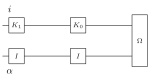
Reading from \(\Omega \) on the right, \(K_0\otimes I\) acts first and \(K_1\otimes I\) acts second. Thus the displayed output is \(\Psi (x)=(K_1\otimes I)(K_0\otimes I)\Omega \).
For a qubit example, take \(X=V\), \(b=1\), \(a_0=a_1=2\), \(x_0=|0\rangle \! \langle 0|\) and \(x_1=|+\rangle \! \langle +|\), where \(|+\rangle =(|0\rangle +|1\rangle )/\sqrt2\). Then
The product order matters: \((K_1K_0)_{01}=-1/4\), whereas \((K_0K_1)_{01}=-1/8\). The complementary space is \(\mathbb {C}\) in this example, so the lower identities are scalar identities.
The set \(\mathcal D\) is compact and nonempty. Each \(L_j\) and the objective \(F\) are continuous on \(\mathcal D\).
In finite dimension, the positive semidefinite trace-one matrices form a compact set. Their finite product is compact. Since \(\| \Omega \| =1\), some global configuration has a nonzero coefficient in \(\Omega \). Restricting that configuration to each region gives \(d_j=\dim \mathcal H_{X_j}{\gt}0\). The densities \(I_{X_j}/d_j\) prove nonemptiness. For \(b{\gt}0\), the shifted matrices are positive definite, and their fixed real powers vary continuously. Identity extension, finite ordered multiplication, evaluation on \(\Omega \), and the norm preserve continuity.
Suppose \(a_j\ge 0\) for every \(j\). For every \(x\in \mathcal D\), every \(j\), and every \(\xi \in \mathcal H_V\),
Consequently, every \(x\in \mathcal D\) satisfies
A positive semidefinite trace-one matrix satisfies \(0\le x_j\le I\). The eigenvalues of \(x_j+bI\) therefore lie in \([b,1+b]\). The negative power has operator norm at most \(b^{-a_j/2}\), while its inverse has norm at most \((1+b)^{a_j/2}\). Applying the identity-extension inequality to the factor and its inverse gives the upper and lower bounds, and applying these bounds successively in the order \(L_0,\ldots ,L_{m-1}\) with \(\| \Omega \| =1\) gives the objective bounds without exchanging any two factors.
Define the minimum value and normalized output by
Under the nonnegative-weight hypothesis, the preceding theorem makes this normalization well defined for every feasible tuple.
There exists \(x_*\in \mathcal D\) such that \(F(x_*)\le F(x)\) for all \(x\in \mathcal D\). Every minimizer in \(\mathcal D\) has objective value \(N\). If all \(a_j\ge 0\), then
At every minimizer \(x_*\in \mathcal D\), \(\widehat\Psi (x_*)=N^{-1}M(x_*)\Omega \).
A continuous real-valued function on a nonempty compact set attains its minimum. The value at any minimizing point is the least element of \(F(\mathcal D)\), hence its infimum. Evaluating the bounds for every feasible tuple at a minimizer gives the bounds on \(N\); positivity permits division by \(F(x)\), and at a minimizer this divisor equals \(N\).
Assume all \(a_j\ge 0\) and set \(b=e^{-R}\). For every real \(R\) and every feasible tuple \(x\),
For \(R\ge 0\), the minimum satisfies
Substituting \(b=e^{-R}{\gt}0\) gives the first display; if \(R\ge 0\), then \(1+e^{-R}\le 2\), so the nonpositive exponent \(-A/2\) gives \((1+e^{-R})^{-A/2}\ge 2^{-A/2}\).
The argument allows empty or repeated regions, zero weights, and singular densities. Neither nestedness of the regions nor commutation of their filters is required. It gives the same minimum value for every minimizer, without asserting uniqueness or smooth dependence of a minimizer on \(R\).
Assume all \(a_j\ge 0\). Then \(\log N\) is the attained minimum of \(x\mapsto \log F(x)\) on \(\mathcal D\).
At any feasible minimizer \(x_*\), one has \(F(x_*)=N{\gt}0\) and \(N\le F(x)\) for every \(x\in \mathcal D\). Monotonicity of the logarithm on the positive real numbers gives \(\log N\le \log F(x)\), with equality at \(x_*\).
In the first-head expansion of the proof of Proposition 4.1, let \(X_0\subseteq \cdots \subseteq X_{m-1}\), let \(a_j\ge 0\) and \(b{\gt}0\), put \(A=\sum _ja_j\), and let \(\Omega \) be a unit vector. For every \(x\in \mathcal D\) there are subspaces \(S_j\subseteq \mathcal H_{X_j}\) with \(\dim S_j\le 1/b\) and a vector \(v\in \sum _j\mathcal C_{X_j}(S_j)\) such that
The tuple \(x\) need not be a minimizer, and repeated regions, zero weights, singular densities, and \(m=0\) are admitted.
Splitting \((x_j+bI)^{a_j/2}=H_j+T_j\) into the spectral part on eigenvalues of \(x_j\) at least \(b\) and the remaining part gives \(\operatorname {rank}H_j\le 1/b\) and \(\| T_j\| \le (2b)^{a_j/2}\) because \(x_j\) has trace one. The product \((x_0+bI)^{a_0/2}\cdots (x_{m-1}+bI)^{a_{m-1}/2}\) inverts the filter product \(M(x)\), so \(\Omega \) is this product applied to \(\Psi (x)\). Writing \(G_j=H_j+T_j\) and expanding according to the first index \(j\) at which a head occurs gives
The preceding tails act inside \(X_j\) because the regions are nested, so the \(j\)th term lies in the cylinder over the range \(S_j\) of \(T_0\cdots T_{j-1}H_j\) on \(X_j\), whose dimension is at most \(\operatorname {rank}H_j\). The remaining term contains only tails and has norm at most \((2b)^{A/2}\| \Psi (x)\| \), which gives (164).
39.15 Continuity of the regularized minimum
Retain the finite regions, independent density tuples and original unit vector of Definition 39.14.1. For each real \(R\), put \(b(R)=e^{-R}\) and write
Here \(L_j(R,x)\) is the identity extension of \((x_j+e^{-R}I_{X_j})^{-a_j/2}\). The feasible set \(\mathcal D\) is fixed as \(R\) varies. The continuity needed in the minimum-growth argument also follows directly from compactness.
For arbitrary real weights \(a_j\), the function \(N:\mathbb {R}\to \mathbb {R}\) is continuous.
For every feasible tuple \(x\) and real \(R\), the matrix \(x_j+e^{-R}I_{X_j}\) is positive definite. Its fixed real power varies jointly continuously with \((R,x)\). Identity extension, ordered multiplication, evaluation on \(\Omega \), and the norm preserve this continuity. Since \(\mathcal D\) is a fixed compact nonempty set, the minimum of the jointly continuous objective varies continuously with \(R\). No choice of a minimizing tuple as a function of \(R\) is required.
If \(a_j\ge 0\) for every \(j\), then \(R\mapsto \log N(R)\) is continuous on \(\mathbb {R}\).
The minimum is continuous and strictly positive at every real radius. Composition with the logarithm gives the assertion.
The regions may be empty or repeated and need not be nested. The argument does not require commutation of the filters. It establishes continuity; the uniform Lipschitz estimate and local absolute continuity in the manuscript are separate assertions.
39.16 Regularity of the logarithmic patch minimum
Let \(V\) be a finite ordered set with arbitrary finite local configuration sets \(A_v\), and put \(\mathcal H_X=\ell ^2(\prod _{v\in X}A_v;\mathbb {C})\). Fix arbitrary regions \(X_0,\ldots ,X_{m-1}\), nonnegative weights \(a_j\), and a unit vector \(\Omega \in \mathcal H_V\). For the feasible independent density tuples \(x\in \mathcal D\) of Definition 39.14.1, write
The minimum is positive and attained. No nesting or commutation is required. The common Lipschitz estimate applies before taking the minimum.
Let \(T\ge 0\) and put \(K=\frac{\kappa }{2}\, 2^{\kappa /2}e^{\kappa T/2}\). Then \(K\ge 0\) and \(\log N\) is \(K\)-Lipschitz on \([0,T]\). In particular, for \(s,t\in [0,T]\),
Zero weights, repeated regions and the empty product are included.
For every feasible \(x\), the derivative of \(\log F_x\) exists throughout \([0,T]\) and has absolute value at most \(K\). The mean value theorem makes every such branch \(K\)-Lipschitz. The logarithmic minimum is attained. Choosing a minimizing tuple at \(t\) gives \(\log N(s)-\log N(t)\le K|s-t|\); interchanging \(s\) and \(t\) gives the reverse inequality. No regularity of the minimizing tuples is needed.
Under the same hypotheses, \(\log N\) is absolutely continuous on \([0,T]\). This includes \(T=0\) and \(\kappa =0\).
A Lipschitz function on a compact real interval is absolutely continuous. Since \(T\ge 0\), the interval with endpoints \(0\) and \(T\) is \([0,T]\).
39.17 Choice of the patch energy parameter
The patch energy estimate has the form \(\langle \phi ,H\phi \rangle -E_0\le C_E\kappa ^2\), where \(C_E=36q^2J\) depends only on the fixed physical parameters. The following scalar choice depends only on \(q\), \(J\) and \(\Delta \), and is made before the regions, radius and minimizing densities are chosen. It does not establish the energy estimate itself.
For an integer \(q\ge 0\) and reals \(J,\Delta \), put \(C_E=36q^2J\) and
where the square root is read as zero when \(C_E=0\).
Let \(J\ge 0\) and \(\Delta \ge 0\), and let \(\kappa =\kappa (q,J,\Delta )\) be the filter exponent (166). Then \(\kappa \le 1/2\), and every \(0\le \kappa '\le \kappa \) satisfies
If \(C_E{\gt}0\) and \(\Delta {\gt}0\), in particular if \(q\ge 1\) and \(J,\Delta {\gt}0\), then \(\kappa {\gt}0\).
The first entry of the minimum gives \(\kappa \le 1/2\). If \(C_E=0\), the energy bound reads \(0\le \Delta /1024\). If \(C_E{\gt}0\), then \(\kappa '^2\le \kappa ^2\le \Delta /(1024C_E)\) by the second entry. Both entries are positive when \(C_E,\Delta {\gt}0\).
For interactions of range \(R\), an extension beyond the source, the same choice is made with the coefficient \(C_E(q,R,J)\) of Definition 39.18.22 in place of \(36q^2J\).
For integers \(q,R\ge 0\) and reals \(J,\Delta \), put
where the square root is read as zero when \(C_E(q,R,J)=0\).
Let \(J\ge 0\) and \(\Delta \ge 0\). Then \(\kappa _R\le 1/2\), and every \(0\le \kappa '\le \kappa _R\) satisfies \(C_E(q,R,J)\kappa '^2\le \Delta /1024\). If \(q,R\ge 1\) and \(J,\Delta {\gt}0\), then \(\kappa _R{\gt}0\).
As in Lemma 39.17.2, with \(C_E(q,R,J)\ge 0\) in place of \(36q^2J\).
This is the parameter choice in the patch construction. The conversion of a proved excess-energy bound into marginal trace-norm bounds uses the original full-system gap and is a separate result.
39.18 Coordinate variation and final-state marginals
Retain the regions, identity extensions, and ordered product of Definition 39.14.1. Write \(K_j=(x_j+bI_{X_j})^{-a_j/2}\), so \(L_j=\widehat{K_j}_{X_j}\). The coordinate variation below is the unstripped first variation in the proof of the regularized patch estimate. Its marginals are those of the same final normalized vector defined in the variational problem.
Fix an index \(j\) and a unitary \(U\) on \(\mathcal H_{X_j}\). Define \(x^{j,U}\) by replacing \(x_j\) with \(Ux_jU^*\) and leaving every other coordinate unchanged. Put
Empty products are identities. The map \(\mathcal I_j\) is complex linear, and \(\mathcal I_j(K_j)=\Psi (x)\). For \(B^*=-B\) and real \(t\), the exponential \(U(t)=e^{tB}\) is unitary. Equal regions at different indices still have independent coordinates.
For \(x\in \mathcal D\), \(b{\gt}0\), arbitrary real weights, and a unitary \(U\) on \(\mathcal H_{X_j}\), one has \(x^{j,U}\in \mathcal D\) and
Unitary conjugation preserves positivity and trace. It fixes the identity, so \(Ux_jU^*+bI=U(x_j+bI)U^*\). Unitary covariance of the real power gives (169). Every factor except the one at index \(j\) is unchanged, giving (170). The argument also applies to singular \(x_j\) because \(x_j+bI\) is positive definite on the full regional space.
Let \(x\in \mathcal D\), \(b{\gt}0\), and \(B^*=-B\) on \(\mathcal H_{X_j}\). For arbitrary real weights, the filtered output satisfies
If \(F(x)\le F(y)\) for every \(y\in \mathcal D\), then
Set \(D_j=\widehat{BK_j-K_jB}_{X_j}\) and \(\Delta _j=P_j^+D_jP_j^-\Omega \). Every line in the following diagram carries the full space \(\mathcal H_V\).

Starting at \(\Omega \) on the right, \(P_j^-\) acts first, \(D_j\) second, and \(P_j^+\) last. The two outer products need not be supported on \(X_j\).
Differentiate \(e^{tB}K_je^{-tB}\) at zero to obtain \(BK_j-K_jB\). Apply the continuous linear map \(\mathcal I_j\) to obtain (171). The entire real curve is feasible. Thus \(t\mapsto \| \Psi (x^{j,e^{tB}})\| ^2\) has a local minimum at zero, and its derivative there is \(2\operatorname {Re}\langle \Psi (x),\mathcal I_j(BK_j-K_jB)\rangle \). Fermat’s theorem gives (172).
Let \(V\) be a finite ordered set with finite local configuration sets \(A_v\), and write \(\mathcal H_X=\ell ^2(\prod _{v\in X}A_v;\mathbb {C})\). Fix regions \(X_0,\ldots ,X_{m-1}\subseteq V\), real weights \(a_j\), positive semidefinite matrices \(x_j\) on \(\mathcal H_{X_j}\), and \(\Omega \in \mathcal H_V\). A hat denotes extension by the identity outside the indicated region. For \(r\in \mathbb {R}\), put \(K_j(r)=(x_j+e^{-r}I_{X_j})^{-a_j/2}\) and define
Then \(\Psi \) is differentiable at every \(R\in \mathbb {R}\), with
The matrices \(x_j\) need not have trace one, and the weights may have either sign. Regions may repeat and need not be nested. For \(m=0\), the product is the identity, the sum is zero, and \(\Psi (r)=\Omega \). This is the ordered product rule underlying the radius derivative estimate for regularized patches.
Since \(x_j+e^{-R}I\) is positive definite, differentiating its real power gives \(K_j'(R)=(a_j/2)e^{-R}(x_j+e^{-R}I)^{-a_j/2-1}\). Extension by the identity is linear. Apply the product rule in the fixed order \(m-1,\ldots ,0\) and then apply each term to \(\Omega \). The term indexed by \(j\) replaces only that occurrence of the factor, giving (174).
Identify configurations indexed by the full region \(V\) with global configurations by forgetting the redundant membership condition. This bijection induces a unitary coordinate identification \(J\). For the same final vector \(\phi =\widehat\Psi (x)\) and every region \(X\subseteq V\), define
At a feasible minimizer with nonnegative weights, \(\phi =N^{-1}M(x)\Omega \). No intermediate filtered vector enters (175).
Let \(V\) be a finite ordered set, let \(n_v\in \mathbb {N}\), and write \(\mathcal H_X=\ell ^2(\prod _{v\in X}[n_v];\mathbb {C})\). For regions \(X_0,\ldots ,X_{m-1}\subseteq V\), real numbers \(a_j\), and matrices \(x_j\in \operatorname {End}(\mathcal H_{X_j})\), define
Every occurrence of a region is retained independently. When \(m=0\), the list is empty.
Let \(V\) be a set, let \(n_v\in \mathbb {N}\), and let \(D_j\subseteq V\) be finite for \(0\leq j{\lt}m\). Write \(\mathcal H_{D_j}=\ell ^2(\prod _{v\in D_j}[n_v];\mathbb {C})\). For \(a_j,b\in \mathbb {R}\) and \(x_j\in \operatorname {End}(\mathcal H_{D_j})\), put \(K_j=(x_j+bI)^{-a_j/2}\) and \(\mathcal L=[(D_{m-1},a_{m-1},x_{m-1}),\ldots ,(D_0,a_0,x_0)]\). Real matrix powers use the nonnegative spectral functional calculus, with value zero when the matrix is not positive semidefinite. If \(F_b(D,a,x)=(D,(x+bI)^{-a/2})\) and \(F_b[\mathcal L]\) denotes application to each entry in its given order, then
Thus this is the list of all filters in decreasing index order. Repeated regions retain their separate occurrences, and both lists are empty when \(m=0\).
Applying a function to each entry commutes with reversing a finite list. The entry with index \(j\) is \((D_j,K_j)\) on both sides.
Let \(J\) be the canonical unitary identification of full-region and global configurations. For arbitrary \(b\in \mathbb {R}\) and an arbitrary vector \(\Omega \), put \(K_j=(x_j+bI)^{-a_j/2}\). Real powers use the nonnegative spectral functional calculus, with value zero when the matrix is not positive semidefinite. Let \(\widehat K_j\) and \(\widetilde K_j\) be the identity extensions in the two coordinate spaces. Then
In particular, the two ordered outputs have the same norm. Empty products are identities. The regions need not be nested or distinct, and the vector need not have unit norm. This identifies the two coordinate descriptions of the ordered product in the regularized patch problem.
Regional basis relabelling gives \(J\widehat K_jJ^{-1}=\widetilde K_j\) for each \(j\). Conjugation preserves the ordered matrix product. Applying the resulting identity to \(J\Omega \) proves the vector identity. Taking norms and using unitarity of \(J\) gives equality of the objectives.
Fix regions \(X_0,\ldots ,X_{m-1}\subseteq V\), real numbers \(a_j,b\), and a vector \(\Omega \). Write \(F(y)\) for the ordered patch objective and let \(x_j\in \operatorname {End}(\mathcal H_{X_j})\) be arbitrary matrices. Suppose that \(F(x)\le F(y)\) for every tuple of density matrices \(y_j\) on the corresponding regions. For a list \(\mathcal L\) of patch factors, let \(P_b(\mathcal L)\) denote the ordered product of its extended filters. Then every list \(\mathcal L'\) of density-matrix factors with the same regions and exponents as \(\mathcal L(x)\), in the same positions, satisfies
Repeated regions retain independent density matrices. The assertion includes the empty list and vanishing outputs. This is the ordered-list form of the minimization in the regularized patch problem.
Enumerate \(\mathcal L'\) in reverse order. Equality of the region lists first gives its length \(m\), and equality of the region and exponent lists then identifies each position. Thus \(\mathcal L'=\mathcal L(y)\) for a tuple of density matrices \(y_j\). Equality of the objective norms gives
Retain arbitrary matrices \(x_j\), real exponents \(a_j\), a real shift \(b\), and an arbitrary input \(\Omega \). Let \(\Psi \) and \(\widetilde\Psi =J\Psi \) be the two ordered outputs. Define \(\widehat\Psi =\| \Psi \| ^{-1}\Psi \) and \(\widehat{\widetilde\Psi }=\| \widetilde\Psi \| ^{-1}\widetilde\Psi \), with both normalizations equal to zero when the output vanishes. Then \(J\widehat\Psi =\widehat{\widetilde\Psi }\).
Linearity and preservation of the norm give
The identity also holds at zero.
For the same arbitrary data and every region \(R\subseteq V\), the canonical marginal of the normalized ordered output satisfies
The identity includes the empty region and a vanishing output.
Apply the regional coordinate identity with the identity relabelling at every site. The normalized vectors agree by Theorem 39.18.10, and taking their reduced density matrices preserves this equality.
For every global vector \(\xi \), region \(X\), and arbitrary complex operator \(K\) on \(\mathcal H_X\),
In particular, \(\langle \phi ,\widehat K_X\phi \rangle =\operatorname{tr}(\rho _XK)\). Each \(\rho _X\) is positive semidefinite. If \(a_j\ge 0\), \(b{\gt}0\), \(\| \Omega \| =1\), and \(x\in \mathcal D\), then \(\operatorname{tr}\rho _X=1\). These assertions include the empty region.
In regional coordinates, \(\widehat K_X=K\otimes I\) and the reduced matrix is the partial trace of \(|J\xi \rangle \! \langle J\xi |\) over the second factor. The partial-trace identity gives \(\operatorname{tr}(\operatorname {Tr}_{V\setminus X}(P)K)=\operatorname{tr}(P(K\otimes I))\). For \(P=|J\xi \rangle \! \langle J\xi |\) this is (176); no real part or Hermiticity assumption is needed. Partial trace preserves positivity and trace. Finally \(J\) preserves the norm and \(\| \phi \| =1\), so \(\operatorname{tr}\rho _X=1\).
For the sitewise basis relabellings of Theorem 35.1.2.4, the marginal \(\rho _X\) of the same final vector \(\phi =\widehat\Psi (x)\) satisfies
This identity holds for every tuple \(x\) and every choice of weights and regulator.
Let \(V\) be a finite set with finite-dimensional complex Hilbert spaces \(\mathcal H_v\), and let \(X_0\subseteq \cdots \subseteq X_{m-1}\subseteq V\). For each \(k\), let \(x_k\) be a positive semidefinite operator on \(\mathcal H_{X_k}\) and let \(a_k\in \mathbb {R}\). Fix \(b{\gt}0\) and an arbitrary vector \(\Omega \in \mathcal H_V\). Set
Put \(\phi =F^{-1}\Psi (x)\) when \(F{\gt}0\), and \(\phi =0\) when \(F=0\). Let \(\rho _k\) be the canonical marginal of \(\phi \) on \(X_k\). Fix \(0\leq j{\lt}m\) and suppose that \([K_k,\rho _k]=0\) for every \(k{\gt}j\). For every complex operator \(H\) on \(\mathcal H_{X_j}\), the insertion
satisfies
Empty products are identities. The operators \(x_k\) need only be positive semidefinite, and the weights \(a_k\) may be arbitrary real numbers. This is the trace calculation used in the proof of [ 287 , Proposition 4.1 ] , before taking the real part in the unitary and diagonal variations.
If \(F=0\), then \(\Psi (x)=0\) and both sides of (178) vanish. Suppose that \(F{\gt}0\). Every \(K_k\) is positive definite and invertible, and so is its identity extension \(L_k\). Set \(A=L_{m-1}\cdots L_{j+1}\) and \(Y=\widehat{H K_j^{-1}}_{X_j}\). Cancellation in the ordered product gives \(\mathcal I_j(H)=A Y A^{-1}\Psi (x)\). Since \(\Psi (x)=F\phi \) and \(F\) is real,
Choose sitewise orthonormal coordinates; the marginal transforms by the same unitary relabelling, preserving the trace pairing. If \(T\) is an operator on \(\mathcal H_{X_k}\) and \(k{\gt}j\), the regional expectation identity, cyclicity of the trace, and \([K_k,\rho _k]=0\) give
Apply this identity successively for \(k=m-1,m-2,\ldots ,j+1\). At each step the remaining conjugated operator is supported on \(X_k\), because all its factors are supported on regions contained in \(X_k\). It follows that \(\langle \phi ,A Y A^{-1}\phi \rangle =\langle \phi ,Y\phi \rangle =\operatorname {Tr}(\rho _j H K_j^{-1})\), which proves the assertion.
Let \(V\) be a finite ordered set with finite local configuration sets \(A_v\), and put \(\mathcal H_X=\ell ^2(\prod _{v\in X}A_v;\mathbb {C})\). Let \(X_0\subseteq \cdots \subseteq X_{m-1}\subseteq V\), let \(a_j\geq 0\), and let \(x_j\) be density matrices on \(\mathcal H_{X_j}\). Fix a unit vector \(\Omega \in \mathcal H_V\). For \(r\in \mathbb {R}\), define
where a hat denotes extension by the identity. Let \(\rho _j(r)\) be the reduced density matrix of \(\Psi (r)/F(r)\) on \(X_j\). Suppose that, at a fixed \(R\in \mathbb {R}\),
Then
Regions may repeat, the matrices \(x_j\) may be singular, and zero weights and the empty product are allowed. The tuple \((x_j)\) is fixed as \(r\) varies. This conditional identity is the trace computation in the radius argument for regularized patches.
The positive shifts make every factor invertible, so \(F(r){\gt}0\). Differentiate \(\frac12\log \| \Psi (r)\| ^2\) and apply the ordered insertion formula. For the term at position \(j\), the assumed commutations and nested regions give the insertion trace identity. Writing \(b=e^{-R}\), the inserted local derivative followed by \(K_j(R)^{-1}\) is \((a_j/2)b(x_j+bI)^{-1}\). The common factor \(F(R)^2\) cancels the denominator from differentiating the logarithm, yielding (179).
Let \(V\) be a finite ordered set with finite local configuration sets \(A_v\), and write \(\mathcal H_X=\ell ^2(\prod _{v\in X}A_v;\mathbb {C})\). Fix regions \(X_0,\ldots ,X_{m-1}\subseteq V\), nonnegative weights \(a_j\), and a unit vector \(\Omega \in \mathcal H_V\). Put \(\kappa =\sum _j a_j\). For density matrices \(x_j\) on \(\mathcal H_{X_j}\), define
where a hat denotes extension by the identity outside the indicated region. If \(T\geq 0\), then for every feasible tuple \(x\) and every \(R\in [0,T]\), the derivative of \(\log F_x\) exists at \(R\) and satisfies
No nesting or commutation is required. The bound includes repeated regions, singular densities, zero weights and the empty product. Source: the uniform local Lipschitz estimate for regularized patches.
Fix \(x\) and \(R\), and put \(b=e^{-R}\) and \(c=\kappa /2\). The positive shift makes all filters invertible, so \(F_x(R){\gt}0\). For \(K_j=(x_j+bI)^{-a_j/2}\) and \(D_j=(a_j/2)b(x_j+bI)^{-a_j/2-1}\), the spectral bounds give
Extension by the identity preserves these upper bounds. Apply the ordered insertion formula and estimate each product in its original order. Summing over its positions yields \(\| \Psi _x'(R)\| \leq c b^{-c}\). The lower norm bound is \(F_x(R)\geq (1+b)^{-c}\). Differentiating \(\frac12\log \| \Psi _x(r)\| ^2\) and using Cauchy–Schwarz therefore gives
Since \(R\leq T\) and \(T\geq 0\), one has \(1+e^R\leq 2e^T\). Raising this inequality to the nonnegative power \(c\) proves (182). No division by a weight is used.
Fix a coordinate \(j\) and a unitary \(U\) on \(\mathcal H_{X_j}\). For a real vector \(y=(y_i)\) indexed by an orthonormal basis of this space, let \(x[y]\) agree with \(x\) at every coordinate except \(j\), and set
The factors in \(F\) retain their original order and act on the original vector \(\Omega \). This is the diagonal variation in the proof of Proposition 4.1.
Let \(b{\gt}0\), let \(x\in \mathcal D\) minimize \(F\) on \(\mathcal D\), and suppose that \(x_j=U\operatorname {diag}(s)U^*\). For every \(y\) with \(y_i\ge 0\) for all \(i\) and \(\sum _i y_i=1\), one has
The weights may be arbitrary real numbers, and \(\Omega \) may be any vector, including zero.
If \(y\) belongs to the probability simplex, then \(U\operatorname {diag}(y)U^*\) is positive semidefinite and has trace \(\sum _i y_i=1\). Hence \(x[y]\in \mathcal D\). The diagonal expression for \(x_j\) gives \(x[s]=x\), so minimality yields \(0\le F(x[s])=F(x)\le F(x[y])\). Squaring gives (187).
Let \(X_0\subseteq \cdots \subseteq X_{m-1}\), let \(a_j{\gt}0\) and \(b{\gt}0\), and let \(\Omega \) be a unit vector. Suppose that \(x\in \mathcal D\) minimizes \(F\) on \(\mathcal D\). Write \(\rho _j\) for the marginal on \(X_j\) of the normalized output \(\Psi (x)/\| \Psi (x)\| \). For every \(j\), there are a unitary \(U_j\), real families \(s_j,p_j\), and a scalar \(0{\lt}\lambda _j\leq 1\) such that
Repeated regions retain independent density variables. This is the clipped spectral formula in the proof of Proposition 4.1.
The indexed minimum gives a minimum over ordered factor lists by Theorem 39.18.9, and Theorem 39.18.11 identifies their normalized marginals. Stationarity of the ordered patch objective and the first-order inequalities for normalized patch outputs in the companion volume [ 253 , “Stationarity of the ordered patch objective” and “First-order inequalities for normalized patch outputs” ] therefore give \(x_j\rho _j=\rho _jx_j\) and
for every density matrix \(y\) commuting with \(x_j\). Both \(x_j\) and \(\rho _j\) are positive semidefinite with trace one. The clipped joint-eigenvalue theorem in the companion volume [ 253 , “Clipped joint eigenvalues” ] , applied to (189), gives (188) and \(0{\lt}\lambda _j\leq 1\).
Let \(X_0\subseteq \cdots \subseteq X_{m-1}\), let \(a_j{\gt}0\) and \(b{\gt}0\), and let \(\Omega \) be a unit vector. Suppose that \(x\in \mathcal D\) minimizes \(F\) on \(\mathcal D\), and write \(\rho _j\) for the marginal on \(X_j\) of the normalized output \(\Psi (x)/\| \Psi (x)\| \). For every \(j\), the filter \(K_j=(x_j+bI_{X_j})^{-a_j/2}\) commutes with \(\rho _j\), and there are a unitary \(W_j\) and real families \(l_j,p_j\) with all \(l_{j,i}{\gt}0\) such that
whenever \(p_{j,i}{\gt}0\) and \(p_{j,k}{\gt}0\). Repeated and empty regions are admitted. This is the logarithmic ratio estimate in the proof of Proposition 4.1.
Theorem 39.18.19 gives a unitary \(U_j\) diagonalizing \(x_j\) and \(\rho _j\) together, with \(s_{j,i}+b=\max \{ p_{j,i}/\lambda _j,b\} \) and \(0{\lt}\lambda _j\le 1\). Hence \(K_j\) is diagonal in the same basis with positive eigenvalues \(l_{j,i}=(s_{j,i}+b)^{-a_j/2}\), and it commutes with \(\rho _j\). The function \(t\mapsto \log \max \{ t/\lambda _j,b\} \) changes by at most \(|\log t-\log t'|\) between positive arguments \(t,t'\). Multiplying by \(a_j/2\) gives (190).
Let \(H\) be an original square Hamiltonian with interaction bound \(J\ge 0\), and let \(\Delta {\gt}0\). Let \(\Omega \) be a unit vector and \(E_0\) a real number with \(H\Omega =E_0\Omega \) and \(H-E_0I\ge \Delta (I-|\Omega \rangle \langle \Omega |)\). Fix an order on the sites of the integer domain, a centre \(c\), and reals \(u\ge 4\), \(0{\lt}\kappa \le 1\) and \(b{\gt}0\). Use the nested patches \(X_j=K(c,r_j)\), \(0\le j{\lt}m\), with the equal weights \(a_j=\kappa /m\) and the input vector \(U\Omega \). If \(x\in \mathcal D\) minimizes \(F\) on \(\mathcal D\) and \(\phi =\widehat\Psi (x)\), then
Repeated clipped patches retain independent densities, and no density is assumed nonsingular. This is the energy bound in the proof of Proposition 4.1.
The weights are positive, so \(\phi \) is a unit vector, and they are at most one. Write \(H_{\mathrm{int}}\) as a sum of Hermitian site and edge terms \(T_i\), supported on single sites or edges \(D_i\), with \(\| T_i\| \le J\). The filters are invertible, so \(\phi \) is the normalized image of the gapped ground vector \(U\Omega \) under the ordered filter product. Each site term crosses no patch, and each edge crosses at most one selected patch. For a term \(T_i\) crossing \(X_j\), let \(d_{ij}=q^{|D_i\cap X_j|}\) be the dimension of its support inside \(X_j\). The logarithmic ratio estimate of Theorem 39.18.20 at that single index, together with \(a_j\le 1\), gives
A crossing edge has exactly one endpoint in \(X_j\), so \(d_{ij}=q\) and the inner sum equals \(q^2J|\partial _\Lambda X_j|\). Hence the right side of (192) equals \(q^2J\sum _ja_j^2|\partial _\Lambda X_j|\), and the quadratic boundary sum bounds this by \(36q^2J\kappa ^2\).
The source treats on-site and nearest-neighbour interactions. The next three entries extend the energy bound to interactions of range \(R\ge 1\), using the patches of Definition 42.20.1.1; they are not in the source. Put \(s_R=2\lceil R/2\rceil \), \(v_R=1+2R(R+1)\) and \(\mu _R=2^{v_R-1}\).
For integers \(q,R\ge 0\) and real \(J\), put
If \(J\ge 0\), then \(C_E(q,R,J)\ge 0\). If \(q,R\ge 1\) and \(J{\gt}0\), then \(C_E(q,R,J){\gt}0\).
Every factor is nonnegative, and positive under the second set of hypotheses, because \(s_R\ge 2\) for \(R\ge 1\).
Let \(J\ge 0\), \(u\ge 0\) and \(0\le j{\lt}m_R\), and index the terms by the nonempty supports \(D\) of graph diameter at most \(R\). Then
A support \(D\) crossing \(K_j\) has a site inside and a site outside, so \(1\le |D\cap K_j|\le |D|-1\le v_R-1\) and \(q^{|D\cap K_j|}\le q^{v_R-1}\), also when \(q=0\). Each of its sites inside \(K_j\) lies in the inner layer \(\mathcal N(c,r_j,R)\), which has at most \(R(16u+4)\) sites, and at most \(\mu _R\) supports contain a given site.
Let \(\Lambda \) be a finite induced lattice domain, \(R\ge 1\) and \(J\ge 0\), and let \(H\) be a Hamiltonian on \(\Lambda \) with one Hermitian term of norm at most \(J\) on each nonempty support of graph diameter at most \(R\). Let \(\Psi \) be a unit vector and \(E_0\) a real number with \(H\Psi =E_0\Psi \) and \(H-E_0I\ge \Delta (I-|\Psi \rangle \langle \Psi |)\). Fix an order on the sites, a centre \(c\), and reals \(u\ge 0\), \(0{\lt}\kappa \le 1\) and \(b{\gt}0\). Use the patches \(X_j=K(c,r_j)\), \(0\le j{\lt}m_R\), of Definition 42.20.1.1, with the equal weights \(a_j=\kappa /m_R\) and the input vector \(\Psi \). If \(x\in \mathcal D\) minimizes \(F\) on \(\mathcal D\) and \(\phi =\widehat\Psi (x)\), then
At \(R=1\) the patches are those of Theorem 39.18.21, which keeps the sharper coefficient \(36q^2J\) for nearest-neighbour interactions.
The argument of Theorem 39.18.21 applies to the terms of \(H\), since each support of graph diameter at most \(R\) is split by at most one patch. It gives (192) with \(d_{ij}=q^{|D_i\cap X_j|}\). Lemma 39.18.24 bounds each inner sum by \(R(16u+4)\mu _Rq^{2(v_R-1)}J\), and (44) bounds \((16u+4)\sum _ja_j^2\) by \(18s_R\kappa ^2\).
Let \(q\ge 0\) be an integer, \(J\ge 0\) and \(\Delta {\gt}0\), and let \(\kappa \) satisfy \(0{\lt}\kappa \le \tfrac 12\) and \(36q^2J\kappa ^2\le \Delta /1024\). For every \(L\), every original square Hamiltonian \(H\) with interaction bound \(J\), every unit vector \(\Omega \) and real \(E_0\) with \(H\Omega =E_0\Omega \) and \(H-E_0I\ge \Delta (I-|\Omega \rangle \langle \Omega |)\), every centre \(c\), and all reals \(u\ge 4\) and \(b{\gt}0\), use the nested patches with equal weights \(a_j=\kappa /m\) and input vector \(U\Omega \). If \(x\in \mathcal D\) minimizes \(F\) on \(\mathcal D\), then every region \(X\) of the integer domain satisfies
where \(\rho _X\) is the marginal of \(\widehat\Psi (x)\). By Lemma 39.17.2, the filter exponent \(\kappa (q,J,\Delta )\) of Definition 39.17.1 is such a parameter when \(q\ge 1\) and \(J{\gt}0\). This is the marginal estimate in the proof of Proposition 4.1.
The energy bound of Theorem 39.18.21 gives \(\operatorname {Re}\langle \phi ,H_{\mathrm{int}}\phi \rangle -E_0\le 36q^2J\kappa ^2\le \Delta /1024\) for the unit vector \(\phi =\widehat\Psi (x)\). The vector \(U\Omega \) is a gapped ground vector of \(H_{\mathrm{int}}\), so the marginal trace-norm estimate of Theorem 39.8.8 gives (196) after the regional coordinate identification.
Let \(q\ge 0\) be an integer, \(J\ge 0\) and \(\Delta {\gt}0\). There is \(0{\lt}\kappa \le \tfrac 12\) with the following property. For every \(L\), every original square Hamiltonian \(H\) with interaction bound \(J\), every unit vector \(\Omega \) and real \(E_0\) with \(H\Omega =E_0\Omega \) and \(H-E_0I\ge \Delta (I-|\Omega \rangle \langle \Omega |)\), every centre \(c\), and all reals \(u\ge 4\) and \(b{\gt}0\), use the nested patches with equal weights \(a_j=\kappa /m\) and input vector \(U\Omega \). If \(x\in \mathcal D\) minimizes \(F\) on \(\mathcal D\), then every region \(X\) of the integer domain satisfies
where \(\rho _X\) is the marginal of \(\widehat\Psi (x)\). The choice of \(\kappa \) depends only on \(q\), \(J\) and \(\Delta \). This is the marginal estimate in the proof of Proposition 4.1.
Let \(q\ge 0\) and \(R\ge 1\) be integers, \(J\ge 0\) and \(\Delta {\gt}0\), and let \(0{\lt}\kappa \le \tfrac 12\) satisfy \(C_E(q,R,J)\kappa ^2\le \Delta /1024\). For every finite induced lattice domain \(\Lambda \), every Hamiltonian \(H\) on \(\Lambda \) with one Hermitian term of norm at most \(J\) on each nonempty support of graph diameter at most \(R\), every unit vector \(\Psi \) and real \(E_0\) with \(H\Psi =E_0\Psi \) and \(H-E_0I\ge \Delta (I-|\Psi \rangle \langle \Psi |)\), every centre \(c\), and all reals \(u\ge 0\) and \(b{\gt}0\), use the patches of Definition 42.20.1.1 with equal weights \(a_j=\kappa /m_R\) and input vector \(\Psi \). If \(x\in \mathcal D\) minimizes \(F\) on \(\mathcal D\), then every region \(X\) of \(\Lambda \) satisfies \(\| \rho _X-\rho _X^{\Psi }\| _1\le \tfrac 1{16}\), where \(\rho _X\) is the marginal of \(\widehat\Psi (x)\). Such a \(\kappa \) exists and depends only on \(q\), \(R\), \(J\) and \(\Delta \); when \(C_E(q,R,J){\gt}0\) the filter exponent \(\kappa _R\) of Definition 39.17.3 is such a parameter. This extends Theorem 39.18.27 to interactions of range \(R\) and is not in the source.
For an integer \(q\) and reals \(J,\Delta ,B_0,p,C_A\), put \(C_S=\max \{ 1,16C_A\} \) and \(C_0=16C_S+\log 8\), and let \(R_0(q,J,\Delta ,B_0,p,C_A)\) be the radius exponent (201) at the constants \(C_0\), \(B_0\), \(p\) and at the filter exponent \(\kappa =\kappa (q,J,\Delta )\). These are the choices of \(C_S\), \(C_Q=16C_S\), \(C_0=C_Q+\log 8\) and \(R_0\) in the proof of Proposition 4.1.
Let \(\Lambda \) be a finite induced lattice domain, \(L\ge 2\), \(B_0,p,\kappa ,C{\gt}0\), \(\Psi \) a unit vector, \(c\) a centre, \(0\le u\le B_0\log L\), and \(r_0\le \dots \le r_{m-1}\) with \(m\ge 1\). Put \(X_j=K(c,r_j)\) and \(a_j=\kappa /m\). Assume \(S_\Psi (X_j)\le C(1+u)\) for every \(j\), and that for every \(b{\gt}0\) every minimizer of \(F\) on \(\mathcal D\) has all marginals within trace distance \(\tfrac 1{16}\) of those of \(\Psi \). Then there are subspaces \(S_j\) of the states on \(X_j\) with \(\dim S_j\le L^{R_0}\), where \(R_0\) is the radius exponent at \(C_0=16C+\log 8\), and a vector \(v\) in the sum of the cylinders \(S_j\otimes \mathcal H_{X_j^c}\) with \(\| \Psi -v\| \le L^{-p}\).
Set \(R=R_0\log L\) and \(b=e^{-R}\). The entropy bound and the marginal closeness give \(\log N(R)\le \frac\kappa 2\bigl(C_0(1+u)+R/4\bigr)\). At a minimizer, the first-head expansion of Theorem 39.14.8 produces subspaces of dimension at most \(1/b=L^{R_0}\) and a vector in the sum of their cylinders within \(N(R)(2b)^{\kappa /2}\) of \(\Psi \), and the radius bounds of Theorem 39.23.2 turn this into \(L^{-p}\).
Let \(q\ge 2\) be an integer, \(J,\Delta {\gt}0\) and \(B_0,p{\gt}0\), and assume the square-grid entropy area law for the ground states of the model at \(J\) and \(\Delta \) with constant \(C_A\). Put \(R_0=R_0(q,J,\Delta ,B_0,p,C_A)\); then \(R_0{\gt}0\). For every \(L\ge 2\), every original square Hamiltonian \(H\) with interaction bound \(J\), every unit vector \(\Omega \) and real \(E_0\) with \(H\Omega =E_0\Omega \) and \(H-E_0I\ge \Delta (I-|\Omega \rangle \langle \Omega |)\), every centre \(c\), and every real \(u\) with \(4\le u\le B_0\log L\), let \(K_0\subseteq \dots \subseteq K_{m-1}\) be the nested patches about \(c\) in the integer square of side \(L\). Then there are subspaces \(S_j\) of the states on \(K_j\) with \(\dim S_j\le L^{R_0}\), and a vector \(v\) in the sum of the cylinders \(S_j\otimes \mathcal H_{K_j^c}\), such that \(\| U\Omega -v\| \le L^{-p}\). This is the cylinder estimate in the proof of Proposition 4.1 with all constants explicit.
Take \(\kappa =\kappa (q,J,\Delta )\), which is admissible in Theorem 39.18.26 by Lemma 39.17.2, and \(C_S=\max \{ 1,16C_A\} \) from Theorem 42.20.1.8. Positivity of \(R_0\) follows from \(\kappa {\gt}0\) and \(C_0\ge 0\). The radii are nondecreasing, so Lemma 39.18.30 applies to the vector \(U\Omega \).
Assume the square-grid entropy area law. Let \(q\ge 2\) be an integer, \(J,\Delta {\gt}0\) and \(B_0,p{\gt}0\). There is \(R_0{\gt}0\) with the following property. For every \(L\ge 2\), every original square Hamiltonian \(H\) with interaction bound \(J\), every unit vector \(\Omega \) and real \(E_0\) with \(H\Omega =E_0\Omega \) and \(H-E_0I\ge \Delta (I-|\Omega \rangle \langle \Omega |)\), every centre \(c\), and every real \(u\) with \(4\le u\le B_0\log L\), let \(K_0\subseteq \dots \subseteq K_{m-1}\) be the nested patches about \(c\) in the integer square of side \(L\). Then there are subspaces \(S_j\) of the states on \(K_j\) with \(\dim S_j\le L^{R_0}\), and a vector \(v\) in the sum of the cylinders \(S_j\otimes \mathcal H_{K_j^c}\), such that
The exponent \(R_0\) is chosen before \(L\), \(H\), \(\Omega \), \(c\) and \(u\). The area law is a hypothesis here; its derivation from the spectral gap is the separate rectangular specialization of the finite-domain area law, which is not yet established. This is the cylinder estimate in the proof of Proposition 4.1.
The area law supplies a constant \(C_A\ge 0\) at \(q\), \(J\), \(\Delta \). Take \(R_0=R_0(q,J,\Delta ,B_0,p,C_A)\) and apply Theorem 39.18.31.
39.19 Stationarity at the original patch minimum
In the finite local coordinates and ordered factors of Definition 39.18.6, let \(X_0\subseteq \cdots \subseteq X_{m-1}\), let \(a_j{\gt}0\) and \(b{\gt}0\), and fix an arbitrary input vector \(\Omega \in \mathcal H_V\). For a feasible tuple of independent regional densities \(x_j\), put
Write \(\phi =\Psi (x)/\| \Psi (x)\| \), using \(\phi =0\) when \(\Psi (x)=0\), and let \(\rho _j\) be its canonical marginal on \(X_j\) as in Definition 39.18.5. The following statement gives the commutation and density order in the stationarity argument at the original norm minimum.
Suppose that \(x\) minimizes \(\| \Psi (x)\| \) over the original feasible set. Then for every \(j\),
Equal regions at different indices retain independent densities.
The reversed list of factors is a descending nested list with positive exponents and feasible density matrices. The canonical coordinate identification preserves its ordered output and norm-minimization comparison. Stationarity of the ordered patch list therefore gives commutation of each \(x_j\) with its final marginal and the displayed density order. The coordinate identity for normalized marginals makes this marginal exactly \(\rho _j\). Finally, \(x_j+bI_{X_j}\) is positive definite. Since it commutes with \(\rho _j\), its real powers commute with \(\rho _j\) as well, giving the assertion for \(K_j\).
No commutation between distinct filters is assumed. The input need not be normalized or nonzero, and the statement includes the empty product.
39.20 The logarithmic derivative at a patch minimum
Let \(V\) be a finite ordered set with local configuration sets \([n_v]\), and write \(\mathcal H_X=\ell ^2(\prod _{v\in X}[n_v];\mathbb {C})\). Fix nested regions \(X_0\subseteq \cdots \subseteq X_{m-1}\), positive weights \(a_j\), and a unit vector \(\Omega \in \mathcal H_V\). In the independent density tuples of Definition 39.14.1, for a feasible tuple \(x\), put
A hat denotes extension by the identity to the complementary sites. Let \(\rho _j(r,x)\) be the marginal on \(X_j\) of \(\Psi _x(r)/F_x(r)\), as in Definition 39.18.5. The derivative is the fixed-tuple identity in the minimum-growth argument.
Fix a real radius \(R\) and a feasible tuple \(x\) minimizing \(F_x(R)\). Keep this tuple fixed as the radius varies. Then \(\log F_x\) is differentiable at \(R\), with
Repeated regions retain independent density matrices. The formula includes the empty product.
Stationarity at the same minimum gives \([K_k(R,x),\rho _k(R,x)]=0\) for every \(k\). These are the commutations required in the ordered logarithmic derivative formula. Applying that formula gives the asserted full derivative of the fixed branch. No family of minimizing tuples is differentiated.
39.21 The regulator trace at a patch minimum
In the setting of the finite local coordinates, nested regions, and positive weights \(a_j{\gt}0\) of Theorem 39.19.1, suppose now that \(\| \Omega \| =1\). For \(b=e^{-R}\), let \(x\) be a feasible minimum of the same ordered norm objective. For an index \(j\), let \(\sigma _j\) be the marginal of the original vector \(\Omega \) on \(X_j\), let \(\rho _j\) be the marginal of the normalized minimizing output, and define \(T_j=b\rho _j(x_j+bI_{X_j})^{-1}\). The next implication isolates the spectral estimate in the regulator argument, taking the entropy and distance bounds as explicit assumptions whose derivation from the physical area law and Hamiltonian gap remains a separate step.
Let \(C{\gt}0\), \(u\ge 0\), and \(R\ge (16C+\log 8)(1+u)\). If \(S(\sigma _j)\le C(1+u)\) and the full trace-norm distance satisfies \(\| \rho _j-\sigma _j\| _1\le \tfrac 1{16}\), then \(\operatorname {tr}T_j\le \tfrac 14\).
Both marginals are density matrices. At \(Q_j=\mathbf1_{[e^{-16C(1+u)},\infty )}(\sigma _j)\), the entropy bound gives
The expectation difference of any effect is bounded by half the full trace-norm distance. Thus \(\operatorname {tr}((I-Q_j)\rho _j)\le \tfrac 1{16}+\tfrac 1{32}\le \tfrac 18\). Stationarity at the minimum gives \([x_j,\rho _j]=0\) and \(\rho _j\le x_j+bI_{X_j}\), hence \(0\le T_j\le bI_{X_j}\) and \(T_j\le \rho _j\). Consequently
The spectral projection is always that of the original marginal; it need not commute with \(\rho _j\) or \(T_j\).
39.22 Growth of the original patch minimum
Let \(V\) be a finite ordered set with local configuration sets \([n_v]\), and fix nested regions \(X_0\subseteq \cdots \subseteq X_{m-1}\), positive weights \(a_j\), and a unit vector \(\Omega \in \mathcal H_V\). In the setting of Definition 39.14.1, write \(F_x(r)\) for the ordered objective norm of a feasible density tuple \(x\in \mathcal D\) at shift \(e^{-r}\), and set \(N(r)=\min _{x\in \mathcal D}F_x(r)\) and \(\kappa =\sum _j a_j\). Denoting by \(\rho _j(r,x)\) the \(X_j\)-marginal of the normalized ordered output, we associate to each feasible minimizing tuple \(x\) the regulator
The two theorems below bound the growth of \(N(r)\) under conditional regulator or entropy-and-distance hypotheses, which a physical application of the minimum-growth argument must verify.
Let \(0\le R_0\le R\). Suppose that for every \(r\in [R_0,R)\), every feasible tuple \(x\) minimizing \(F_x(r)\), and every index \(j\), the regulator satisfies \(\operatorname {Re}\operatorname{tr}T_j(r,x)\le \tfrac 14\). Then, including the cases \(R=R_0\) and \(m=0\),
Write \(g(r)=\log N(r)\). At each \(r\in [R_0,R)\), an attained minimizing tuple \(x\) defines a smooth branch \(\log F_x\) that touches \(g\) at \(r\), satisfies \(g\le \log F_x\) across the interval, and has derivative at \(r\) bounded by \(\sum _j(a_j/2)(1/4)=\kappa /8\). Applying the comparison principle for a continuous lower envelope to these contacting branches gives
Combining this bound with the initial estimate \(g(R_0)\le \kappa R_0/2\) and using \(\kappa R_0\ge 0\) yields
Let \(C{\gt}0\), \(u\ge 0\), and put \(R_0=(16C+\log 8)(1+u)\). Suppose that \(R\ge R_0\) and that the marginal \(\sigma _j\) of the original vector \(\Omega \) satisfies \(S(\sigma _j)\le C(1+u)\) for every \(j\). Suppose also that for every \(r\in [R_0,R)\), every feasible tuple \(x\) minimizing \(F_x(r)\), and every \(j\), the full trace norm \(\| \cdot \| _1\) satisfies
Then
Because \(R_0\ge 0\) and both the entropy bound \(S(\sigma _j)\le C(1+u)\) and the trace-norm bound \(\| \rho _j(r,x)-\sigma _j\| _1\le \tfrac 1{16}\) hold at every \(r\in [R_0,R)\), the regulator trace estimate gives \(\operatorname {Re}\operatorname{tr}T_j(r,x)\le \tfrac 14\) for each minimizing tuple \(x\) and index \(j\). Applying Theorem 39.22.1 with \(R_0=(16C+\log 8)(1+u)\) then yields the stated bound.
39.23 An explicit logarithmic patch radius
The constants in the logarithmic radius can be chosen before the system size. The following estimates are the scalar inequalities in the explicit radius choice and the cylinder count.
For real constants \(C_0,B_0,p,\kappa \), set
Suppose that \(C_0,B_0,p\ge 0\), \(\kappa {\gt}0\), \(L\ge 2\), and \(u\le B_0\log L\). With \(R_0\) as in (201) and \(R=R_0\log L\), one has \(R_0{\gt}0\) and
Put \(A=C_0(B_0+1/\log 2)\). Since \(\log L\ge \log 2{\gt}0\), \(1\le \log L/\log 2\) and \(C_0(1+u)\le A\log L\). The positivity of \(A+1+2p/\kappa \) gives \(R_0{\gt}0\), and \(R_0\ge A\) gives \(C_0(1+u)\le R\). For the remainder bound, substitute (201) into
Let \(B_0\ge 0\), \(L\ge 2\), \(\alpha \in \mathbb {R}\), and \(m\in \mathbb {N}\). If \(m\le (B_0/2)\log L+1\), then \(mL^\alpha \le (1+B_0/2)L^{\alpha +1}\).
The inequalities \(\log L\le L\) and \(1\le L\) give \((B_0/2)\log L+1\le (1+B_0/2)L\). Multiply by \(L^\alpha \ge 0\) and use \(L^{\alpha +1}=L^\alpha L\).